`JOIN` the `DISTINCT` with SQL¶

Outline¶

📊 Why SQL
🎩 Starting SQL with Python (DuckDB + SQL Magic)
🏗️ Structure of a SQL statement
📥 Data Import
🤿 SQL Fundamentals
- Basics: semicolons and comments
- SELECT
- WHERE Clause
- GROUP BY and Aggregates
- HAVING Clause
- JOIN operations
- Subqueries
🚨 Advanced SQL
- Data Modification (UPDATE, INSERT, DELETE)
- Common Table Expressions (CTEs)
- Window functions
- Views and Materialized Views
- Performance optimization
🔄 SQL with Python
- pandas integration
- SQLite
- SQLAlchemy

📊 Why SQL?¶

Data is big¶

SQL (Structured Query Language) is a powerful tool in the data scientist's arsenal, offering a structured and efficient way to interact with databases. It serves as a standard language for managing and querying relational databases, providing a systematic approach to handle vast datasets. Here are some compelling reasons why SQL is a must-have skill for data scientists.

Simplified Data Retrieval¶

SQL allows you to retrieve specific data from large datasets with ease. Its simple syntax enables you to express complex queries succinctly, making it a valuable tool for extracting meaningful insights from databases.

Standardized Language¶

SQL is a standardized language used across different database management systems (DBMS). Whether you're working with MySQL, PostgreSQL, SQLite, or others, the fundamental SQL principles remain consistent. This standardization enhances portability and ensures your skills are transferable across various platforms.

Efficient Data Manipulation¶

With SQL, you can perform various data manipulation tasks, including filtering, sorting, and aggregating data. It provides a robust framework for handling data at scale, making it an essential skill for anyone dealing with large datasets in a professional setting.

Seamless Integration with Python¶

The integration of SQL with Python opens up new possibilities for data scientists. You can leverage the strengths of both SQL and Python by combining SQL's data manipulation capabilities with Python's extensive libraries for analysis, visualization, and machine learning.

🎩 Starting SQL with Python (DuckDB and SQL Magic)¶

SQL Magic with DuckDB¶

The ipython-sql package (reimplemented by jupysql) provides a shortcut (%-commands are called "magic") for querying SQLalchemy within notebooks:

%sql inline queries
%%sql for multi-line queries

# Install required libraries
%pip install pandas duckdb-engine ipython-sql

# Import necessary libraries
import pandas as pd
import duckdb
%load_ext sql

# Create a sample Pandas DataFrame
data = {'ID': [1, 2, 3, 4],
        'Name': ['Alice', 'Bob', 'Charlie', 'David'],
        'Age': [25, 30, 22, 35]}

df = pd.DataFrame(data)

# Connect to DuckDB and load the DataFrame into DuckDB
con = duckdb.connect(database=':memory:', read_only=False)
con.register('sample_data', df)

# Use SQL magic command to query the DuckDB database
%sql duckdb://localhost

# Show the content of the DuckDB database
%sql SELECT * FROM df

Why DuckDB?¶

Embedded database (no server needed)
Columnar storage (perfect for analytics)
Lightning fast for analytical queries
Seamless integration with Python

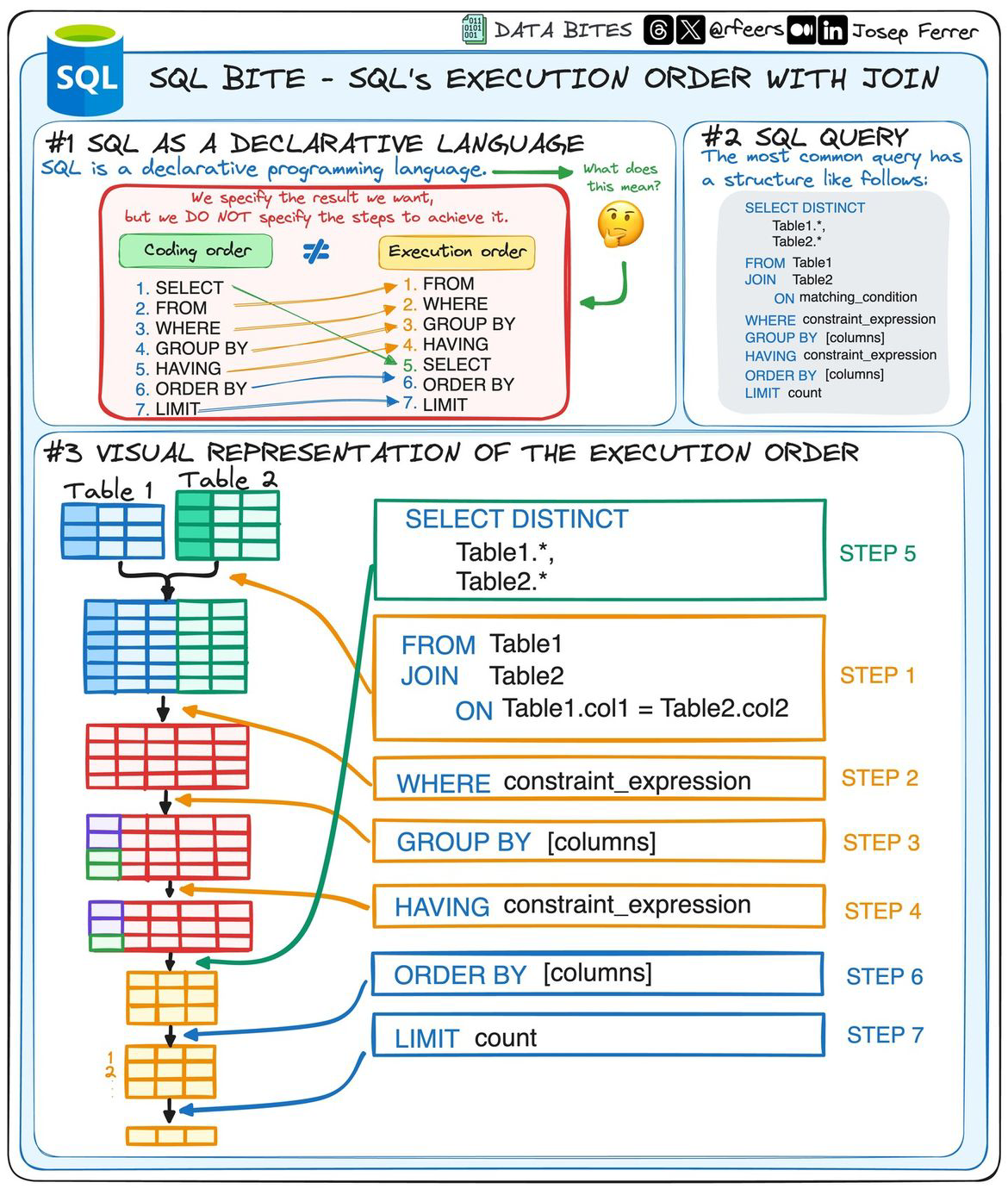
🏗️ Structure of a SQL statement¶

-- Retrieve a list of unique department names and the total number of employees in each department
SELECT DISTINCT department_name, COUNT(employee_id) AS total_employees
FROM employees
JOIN departments ON employees.department_id = departments.department_id
WHERE employees.salary > 50000 -- Filter employees with a salary greater than 50000
GROUP BY department_name
ORDER BY total_employees DESC -- Order the results by total employees in descending order
LIMIT 10; -- Limit the output to the top 10 departments

Explanation of each part:

SELECT DISTINCT:** Selects unique department names.
COUNT(employee_id) AS total_employees:** Counts the number of employees in each department and renames the column as "total_employees."
FROM employees:** Specifies the main table as "employees."
JOIN departments ON employees.department_id = departments.department_id:** Joins the "employees" table with the "departments" table based on the department_id.
WHERE employees.salary > 50000:** Filters out employees with a salary less than or equal to 50000.
GROUP BY department_name:** Groups the results by department_name.
ORDER BY total_employees DESC:** Orders the results by the total number of employees in descending order.
LIMIT 10:** Limits the output to the top 10 departments.

Read SQL the way a computer does¶

Start with the select, then walk through the execution order

SQL Execution Order

📥 Data Import¶

COPY Command¶

The COPY command is the most efficient way to import data into SQL databases. It's much faster than INSERT statements for bulk data loading.

-- Basic COPY syntax
COPY table_name FROM 'file_path' 
WITH (FORMAT csv, HEADER true);

-- Example with NHANES data
COPY demographics FROM 'lectures/03/demo/data/demographics.csv' 
WITH (FORMAT csv, HEADER true, DELIMITER ',');

Key features of COPY:

Direct file import
Support for various formats (CSV, JSON, etc.)
Header handling
Delimiter specification
Error handling options
Data type inference

CREATE TABLE AS COPY¶

You can create and populate a table in one step using CREATE TABLE AS COPY:

-- Create and populate table in one step
CREATE TABLE demographics AS
COPY FROM 'lectures/03/demo/data/demographics.csv'
WITH (FORMAT csv, HEADER true);

-- With explicit column types
CREATE TABLE demographics (
      seqn INTEGER PRIMARY KEY,
      age INTEGER,
      gender TEXT,
      race TEXT,
      education TEXT
) AS COPY FROM 'lectures/03/demo/data/demographics.csv'
WITH (FORMAT csv, HEADER true);

Live demo¶

Demo 1: Setup and Import

🤿 SQL Fundamentals¶

Semicolons `;` and comments `--`¶

SQL statements are separated using semicolons. You may send multiple statements at the same time as long as they are separated by semicolons. NOTE: your environment may expect to receive only a single table as a response, so multiple select statements may NOT be valid.

Unlike python, SQL uses double-dashes to indicate comments. Comments may be on their own lines or on the same line as code.

`SELECT`¶

The SELECT statement is fundamental for retrieving data. It allows you to specify the columns you want to retrieve and the conditions for selecting rows. For example:

SELECT column1, column2
FROM table
WHERE condition;

The SELECT statement is versatile and can be customized to fetch specific columns from a table based on specified conditions.

JOIN Operations¶

JOIN operations combine data from multiple tables based on related columns.

SELECT *
FROM table1
INNER JOIN table2 ON table1.column1 = table2.column2;

JOIN Types¶

INNER JOIN: Returns matching rows from both tables
LEFT JOIN: Returns all rows from left table + matching rows from right
RIGHT JOIN: Returns all rows from right table + matching rows from left
FULL JOIN: Returns all rows from both tables (use with caution!)

Types of JOINs

Important

Always specify JOIN type explicitly to avoid unexpected FULL JOINs!

Filtering and Grouping¶

WHERE Clause¶

The WHERE clause serves as your data gatekeeper, allowing you to filter rows based on specific conditions. It operates before grouping and aggregation, helping you focus on the data that truly matters.

Example:

-- Selecting employees with a salary greater than $50,000
SELECT *
FROM employees
WHERE salary > 50000;

Common WHERE operators:

Comparison: =, >, <, >=, <=, <>
Logical: AND, OR, NOT
Pattern matching: LIKE, ILIKE
Range: BETWEEN, IN
NULL handling: IS NULL, IS NOT NULL

GROUP BY and Aggregates¶

The GROUP BY clause groups rows that have the same values in specified columns into summary rows. It's often used with aggregate functions to perform calculations on each group.

Example:

-- Calculating the total sales for each product category
SELECT category, SUM(sales) AS total_sales
FROM products
GROUP BY category;

Aggregate Functions¶

Aggregate functions perform operations on groups of rows defined by the GROUP BY clause. They summarize the data within each group, providing valuable aggregated results.

Common Aggregate Functions:

COUNT:** Counts the number of rows in each group
SUM:** Calculates the sum of values within each group
AVG:** Computes the average value within each group
MIN:** Finds the minimum value within each group
MAX:** Identifies the maximum value within each group

Example:

-- Multiple aggregates in one query
SELECT 
    department,
    COUNT(*) AS employee_count,
    AVG(salary) AS avg_salary,
    MAX(salary) AS max_salary,
    MIN(salary) AS min_salary
FROM employees
GROUP BY department;

HAVING Clause¶

While the WHERE clause filters individual rows, the HAVING clause steps in after grouping to filter groups based on conditions applied to aggregate values. It's your tool for fine-tuning group-level criteria.

Example:

-- Selecting departments with an average salary greater than $70,000
SELECT department, AVG(salary) AS average_salary
FROM employees
GROUP BY department
HAVING AVG(salary) > 70000;

Key differences between WHERE and HAVING:

WHERE filters rows before grouping
HAVING filters groups after aggregation
HAVING can use aggregate functions
WHERE is more efficient when possible

Putting It All Together¶

You can combine all three clauses to create powerful queries:

-- Complex example combining all clauses
SELECT 
    department,
    COUNT(*) AS employee_count,
    AVG(salary) AS avg_salary
FROM employees
WHERE hire_date > '2020-01-01'  -- Filter rows first
GROUP BY department              -- Group the filtered rows
HAVING COUNT(*) > 5            -- Filter groups after aggregation
ORDER BY avg_salary DESC;      -- Sort the final results

Subqueries¶

Subqueries enable you to nest one query within another. They are useful for complex queries where you need the result of one query as input for another.

SELECT column
FROM table
WHERE column IN (SELECT column FROM another_table WHERE condition);

Subqueries can be used in various parts of a SQL statement, such as the SELECT, FROM, and WHERE clauses.

Subqueries may also be named. This is especially useful in joins

SELECT main_table.column1, main_table.column2, subquery.total_count
FROM main_table
JOIN (
    SELECT related_column, COUNT(*) AS total_count
    FROM related_table
    GROUP BY related_column
) AS subquery ON main_table.column1 = subquery.related_column;

Live demo¶

Demo 2: SQL Basics

🚨 Advanced SQL¶

Data Modification (UPDATE, INSERT, DELETE)¶

These statements are used to modify data in the database. They should be used with caution as they can permanently change your data.

-- UPDATE: Modify existing records
UPDATE table
SET column1 = value1
WHERE condition;

-- INSERT: Add new records
INSERT INTO table (column1, column2)
VALUES (value1, value2);

-- DELETE: Remove records
DELETE FROM table
WHERE condition;

Advanced INSERT Patterns¶

While COPY is preferred for bulk loading, INSERT is useful for:

Adding single rows
Conditional inserts
Data transformation during insert

-- Basic INSERT
INSERT INTO demographics (seqn, age, gender, race)
VALUES (12345, 30, 'M', 'White');

-- INSERT with SELECT
INSERT INTO demographics (seqn, age, gender, race)
SELECT seqn, age, gender, race
FROM temp_table
WHERE age > 18;

-- Conditional INSERT
INSERT INTO demographics (seqn, age, gender, race)
SELECT seqn, age, gender, race
FROM temp_table
WHERE NOT EXISTS (
    SELECT 1 FROM demographics d 
    WHERE d.seqn = temp_table.seqn
);

UPDATE with JOIN¶

You can update records based on joins with other tables:

-- Update employee salaries based on department averages
UPDATE employees e
SET salary = salary * 1.1
FROM departments d
WHERE e.department_id = d.department_id
AND d.name = 'Engineering';

DELETE with Subqueries¶

Complex deletion patterns using subqueries:

-- Delete inactive users who haven't logged in for a year
DELETE FROM users
WHERE user_id IN (
    SELECT user_id 
    FROM login_history 
    WHERE last_login < CURRENT_DATE - INTERVAL '1 year'
);

Common Table Expressions (CTEs)¶

The WITH clause, also known as Common Table Expressions (CTE), allows you to define temporary result sets that can be referenced within the context of a larger query. It enhances the readability and reusability of complex queries.

WITH temp_table AS (
    SELECT column
    FROM another_table
    WHERE condition
)

SELECT *
FROM main_table
JOIN temp_table ON main_table.column = temp_table.column;

Window Functions¶

Window functions operate across a set of table rows related to the current row. They provide a powerful way to perform calculations over a specified range of rows related to the current row. Window functions are typically used in conjunction with the OVER clause, which defines the window or set of rows the function operates on.

-- Example of calculating the running total of sales using a window function
SELECT date, sales, SUM(sales) OVER (ORDER BY date) AS running_total
FROM sales_data;

Common window functions include ROW_NUMBER, RANK, DENSE_RANK, LAG, and LEAD. These functions offer advanced analytical capabilities, allowing you to derive insights from your data that go beyond basic aggregations.

Views and Materialized Views¶

Views are virtual tables that store the result of a query. They can simplify complex queries and provide a layer of abstraction.

-- Create a view
CREATE VIEW employee_departments AS
SELECT e.employee_id, e.name, d.department_name
FROM employees e
JOIN departments d ON e.department_id = d.department_id;

-- Use the view
SELECT * FROM employee_departments;

-- Materialized views store the actual data
CREATE MATERIALIZED VIEW sales_summary AS
SELECT product_id, SUM(quantity) as total_sales
FROM sales
GROUP BY product_id;

-- Refresh materialized view
REFRESH MATERIALIZED VIEW sales_summary;

Performance Optimization¶

Use appropriate indexes
Limit result sets early
Avoid unnecessary subqueries
Consider materialized views for complex queries

Live demo¶

Demo 3: Complex Queries

🔄 SQL with Python¶

pandas Integration¶

Pandas is a widely-used data manipulation library in Python, and Pyarrow serves as a bridge between Pandas and Arrow, a cross-language development platform for in-memory data. This combination allows for efficient conversion and manipulation of large datasets.

Installation¶

Ensure you have both Pandas and Pyarrow installed:

pip install pandas

Using SQL with Pandas¶

Pandas provides a convenient read_sql function that allows you to execute SQL queries and retrieve the results directly into a DataFrame.

import pandas as pd
import pyarrow as pa
import pyarrow.dataset as ds

## Example SQL query
sql_query = "SELECT column1, column2 FROM table WHERE condition;"

## Reading SQL query into Pandas DataFrame
df = pd.read_sql(sql_query, connection)

SQLite¶

SQLite is a lightweight, file-based database engine that is often used for local development and small-scale applications. Python's standard library includes an SQLite module, making it easy to work with SQLite databases. It is ubiquitous, but also not a fully featured as pandas + pyarrow/duckdb.

Using SQLite with Python¶

import sqlite3

## Connecting to an SQLite database (creates a new file if not exists)
conn = sqlite3.connect('example.db')

## Example SQL query
sql_query = "SELECT column1, column2 FROM table WHERE condition;"

## Reading SQL query into Pandas DataFrame
df = pd.read_sql_query(sql_query, conn)

SQLAlchemy¶

When working with larger databases, you may need to connect to external databases. Libraries like SQLAlchemy provide a flexible and efficient way to interact with a variety of databases.

from sqlalchemy import create_engine

## Example connection to a PostgreSQL database
engine = create_engine('postgresql://user:password@localhost:5432/database')
df = pd.read_sql_query(sql_query, engine)

Live demo¶

Demo 4: Python Integration

JOIN the DISTINCT with SQL¶

Outline¶

📊 Why SQL?¶

Data is big¶

Simplified Data Retrieval¶

Standardized Language¶

Efficient Data Manipulation¶

Seamless Integration with Python¶

🎩 Starting SQL with Python (DuckDB and SQL Magic)¶

SQL Magic with DuckDB¶

Why DuckDB?¶

🏗️ Structure of a SQL statement¶

Read SQL the way a computer does¶

📥 Data Import¶

COPY Command¶

CREATE TABLE AS COPY¶

Live demo¶

🤿 SQL Fundamentals¶

Semicolons ; and comments --¶

SELECT¶

JOIN Operations¶

JOIN Types¶

Filtering and Grouping¶

WHERE Clause¶

GROUP BY and Aggregates¶

Aggregate Functions¶

HAVING Clause¶

Putting It All Together¶

Subqueries¶

Live demo¶

🚨 Advanced SQL¶

Data Modification (UPDATE, INSERT, DELETE)¶

Advanced INSERT Patterns¶

UPDATE with JOIN¶

DELETE with Subqueries¶

Common Table Expressions (CTEs)¶

Window Functions¶

Views and Materialized Views¶

Performance Optimization¶

Live demo¶

🔄 SQL with Python¶

pandas Integration¶

Installation¶

Using SQL with Pandas¶

SQLite¶

Using SQLite with Python¶

SQLAlchemy¶

Live demo¶

`JOIN` the `DISTINCT` with SQL¶

Semicolons `;` and comments `--`¶

`SELECT`¶