Classification: Putting a label on things¶

• Quick example
• Classification model types and how to evaluate them
• How things can go wrong…
• … and how to fix it
• Hands-on with code

Preamble¶

1. The Urgency of Interpretability by Dario Amodei (Anthropic founder/CEO) on his blog
2. HuggingFace's Daily Papers by AK
3. Example analytical technical interview - Analytics Technical Interview
4. Example interview take-home - https://github.com/christopherseaman/five_twelve
5. Data sources available on Physionet (some require credentialed access) - https://physionet.org/about/database/
6. Labeling things by hand when everyone's trying not to part of Randy Au's excellent Counting Stuff

git merge conflicts¶

1. Working in branches for each exercise
2. Save to branch and sync (discarding commits)
3. (Optional) Add files from branch back to main through a Pull Request

On the perils of ChatGPT¶

Not exactly what Linus was talking about, but the quote remains relevant…

💥Crash course in classification¶

The building blocks of ML are algorithms for regression and classification:

• Regression: predicting continuous quantities
• Classification: predicting discrete class labels (categories)

Classification methods¶

Conceptual Overview: Classification algorithms learn to assign labels to data points based on their features. In health data, this might mean predicting whether a patient has a disease based on lab results.

Reference Card: Common Classification Methods

• Logistic Regression: Linear model for binary outcomes. Easy to interpret.
• Decision Trees: Tree structure, splits data by feature values. Intuitive but can overfit.
• Random Forest: Many decision trees combined. More robust, less overfitting.
• Support Vector Machines (SVM): Finds the best boundary between classes. Good for complex data.
• Naive Bayes: Probabilistic, assumes features are independent. Fast and simple.
• Neural Networks: Layers of nodes, can model complex patterns. Powerful but less interpretable.

Minimal Example: Logistic Regression in Python

from sklearn.linear_model import LogisticRegression
X = [[1, 2], [2, 3], [3, 4]]
y = [0, 1, 0]
model = LogisticRegression().fit(X, y)
print(model.predict([[2, 2]]))  # Predicts class label

• Some links to dive deeper:
  • A nice tour of methods: https://github.com/bagheri365/ML-Models-for-Classification
  • Cancer classification (Kaggle)
  • Comparison of XGBoost, Random Forest, and Nomograph for Prediction of Disease Severity
  • Prediction Method for Hypertension (Diagnostics Journal)
  • Guide to Predictive Lead Scoring using ML (Towards AI)
  • True end-to-end ML example: Lead Scoring (Towards Data Science)

🧠 Comprehension Checkpoint:

• What is the difference between regression and classification?
• Name two classification algorithms and a scenario where each might be useful in health data.

Model evaluation¶

There are many more classification approaches than data scientists, so choosing the best one for your application can be daunting. Thankfully, all of them output predicted classes for each data point. We can use this similarity to define objective performance criteria based on how often the predicted class matches the underlying truth.

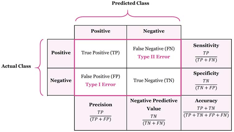
Conceptual Overview: Model evaluation metrics help us understand how well our classifier is performing. In health data, it's especially important to know not just how often the model is right, but how it gets things wrong (e.g., missing a disease vs. a false alarm).

• Precision (Positive Predictive Value) = \(\frac{TP}{TP + FP}\)

  How well it performs when it predicts positive

• Recall (Sensitivity, True Positive Rate) = \(\frac{TP}{TP+FN}\)

  How well it performs among actual positives

• Accuracy = \(\frac{(TP+TN)}{(TP+FP+FN+TN)}\)

  How well it performs among all known classes

• F1 score = \(2 \times \frac{Recall * Precision}{Recall + Precision}\)

  Balanced score for overall model performance

• Specificity (Selectivity, True Negative Rate) = \(\frac{TN}{TN + FP}\)

  Similar to Recall, how well it performs among actual negatives

• Miss Rate (False Negative Rate) = \(\frac{FN}{TP + FN}\)

  Proportion of positives that were incorrectly classified, good measure when missing a positive has a high cost

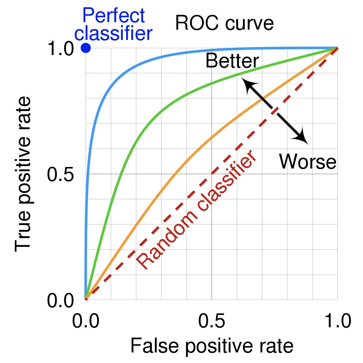
• Receiver-Operator Curve (ROC Curve) and Area Under the Curve (AUC)

  Plot the True Positive vs. False Positive rates, which provides a scale-invariant measure of performance. A random model on balanced class data will have a score of 0.5, while a perfect model will always have a score of 1

Reference Card: confusion_matrix

• Function: sklearn.metrics.confusion_matrix()
• Purpose: Compute confusion matrix to evaluate classification accuracy.
• Key Parameters:
• y_true: (Required) Ground truth (correct) target values.
• y_pred: (Required) Estimated targets as returned by a classifier.
• labels: (Optional, default=None) List of labels to index the matrix. If None, labels that appear at least once in y_true or y_pred are used in sorted order.
• normalize: (Optional, default=None) Normalizes confusion matrix over the true (rows), predicted (columns) conditions or all the population. Can be 'true', 'pred', 'all', or None.

Example:

from sklearn.metrics import confusion_matrix
y_true = [1, 0, 1, 1, 0] # Actual labels
y_pred = [1, 0, 0, 1, 1] # Predicted labels
cm = confusion_matrix(y_true, y_pred)
print(cm)
# Output interpretation (for binary case):
# [[TN, FP],
#  [FN, TP]]

I get in trouble with the data science police if I don't include something about confusion matrices:

• Precision (Positive Predictive Value) = \(\frac{TP}{TP + FP}\)

  How well it performs when it predicts positive

• Recall (Sensitivity, True Positive Rate) = \(\frac{TP}{TP+FN}\)

  How well it performs among actual positives

• Accuracy = \(\frac{(TP+TN)}{(TP+FP+FN+TN)}\)

  How well it performs among all known classes

• F1 score = \(2 \times \frac{Recall * Precision}{Recall + Precision}\)

  Balanced score for overall model performance

• Specificity (Selectivity, True Negative Rate) = \(\frac{TN}{TN + FP}\)

  Similar to Recall, how well it performs among actual negatives

• Miss Rate (False Negative Rate) = \(\frac{FN}{TP + FN}\)

  Proportion of positives that were incorrectly classified, good measure when missing a positive has a high cost

• Receiver-Operator Curve (ROC Curve) and Area Under the Curve (AUC)

  Plot the True Positive vs. False Positive rates, which provides a scale-invariant measure of performance. A random model on balanced class data will have a score of 0.5, while a perfect model will always have a score of 1

ROC curve¶

Conceptual Overview: An ROC curve (Receiver Operating Characteristic curve) shows how a classifier's performance changes as you vary the threshold for predicting "positive." It plots:

• True Positive Rate (TPR) (a.k.a. recall): How many actual positives did we catch?
  • TPR (Recall): \(TPR = TP / (TP + FN)\)
• False Positive Rate (FPR): How many actual negatives did we incorrectly call positive?
  • FPR: \(FPR = FP / (FP + TN)\)

Reference Card: roc_curve

• Function: sklearn.metrics.roc_curve()
• Purpose: Compute Receiver operating characteristic (ROC) curve points.
• Key Parameters:
• y_true: (Required) True binary labels.
• y_score: (Required) Target scores, can either be probability estimates of the positive class or confidence values.
• pos_label: (Optional, default=1) The label of the positive class.
• drop_intermediate: (Optional, default=True) Whether to drop some suboptimal thresholds which would not appear on a plotted ROC curve.

Example:

from sklearn.metrics import roc_curve
y_true = [0, 0, 1, 1]        # Actual labels
y_scores = [0.1, 0.4, 0.35, 0.8] # Model scores/probabilities for class 1
fpr, tpr, thresholds = roc_curve(y_true, y_scores)
print("FPR:", fpr)
print("TPR:", tpr)
# Typically, you'd plot fpr vs tpr using matplotlib

An ROC curve plots TPR vs. FPR at different classification thresholds. Lowering the classification threshold classifies more items as positive, thus increasing both False Positives and True Positives. The following figure shows a typical ROC curve.

Figure 4. TP vs. FP rate at different classification thresholds.

To compute the points in an ROC curve, we could evaluate a logistic regression model many times with different classification thresholds, but this would be inefficient. Fortunately, there's an efficient, sorting-based algorithm that can provide this information for us, called AUC.

AUC/AUROC: Area Under the ROC Curve¶

Conceptual Overview: While the ROC curve visualizes the trade-off between TPR and FPR across different thresholds, the AUC (Area Under the Curve) provides a single number summarizing this performance. It measures the overall ability of a classifier to rank positive cases higher than negative ones across all thresholds. An AUC of 1.0 represents a perfect classifier (covering the entire area), while 0.5 means the model is no better than random guessing (following the diagonal line).

Reference Card: AUC/AUROC

• AUC/AUROC (Area Under the ROC Curve): Probability that a randomly chosen positive is ranked above a randomly chosen negative.
• Range: 0 (worst) to 1 (best); 0.5 = random.

Reference Card: roc_auc_score

• Function: sklearn.metrics.roc_auc_score()
• Purpose: Compute Area Under the Receiver Operating Characteristic Curve (AUC) from prediction scores.
• Key Parameters:
• y_true: (Required) True binary labels.
• y_score: (Required) Target scores, can either be probability estimates of the positive class or confidence values.
• average: (Optional, default='macro') Determines the type of averaging performed on the data for multiclass problems.
• max_fpr: (Optional, default=None) If not None, the standardized partial AUC over the range [0, max_fpr] is returned.

Example:

Figure 5. AUC (Area under the ROC Curve).

AUC provides an aggregate measure of performance across all possible classification thresholds. One way of interpreting AUC is as the probability that the model ranks a random positive example more highly than a random negative example. For example, given the following examples, which are arranged from left to right in ascending order of logistic regression predictions:

Figure 6. Predictions ranked in ascending order of logistic regression score.

AUC represents the probability that a random positive (green) example is positioned to the right of a random negative (red) example.

AUC ranges in value from 0 to 1. A model whose predictions are 100% wrong has an AUC of 0.0; one whose predictions are 100% correct has an AUC of 1.0.

from sklearn.metrics import roc_auc_score
y_true = [0, 0, 1, 1]        # Actual labels
y_scores = [0.1, 0.4, 0.35, 0.8] # Model scores/probabilities for class 1
auc_score = roc_auc_score(y_true, y_scores)
print(f"AUC Score: {auc_score}")  # Output: AUC Score: 0.75

Figure 5. AUC (Area under the ROC Curve).

AUC provides an aggregate measure of performance across all possible classification thresholds. One way of interpreting AUC is as the probability that the model ranks a random positive example more highly than a random negative example. For example, given the following examples, which are arranged from left to right in ascending order of logistic regression predictions:

Figure 6. Predictions ranked in ascending order of logistic regression score.

AUC represents the probability that a random positive (green) example is positioned to the right of a random negative (red) example.

AUC ranges in value from 0 to 1. A model whose predictions are 100% wrong has an AUC of 0.0; one whose predictions are 100% correct has an AUC of 1.0.

AUC is desirable for the following two reasons:

• AUC is scale-invariant. It measures how well predictions are ranked, rather than their absolute values.
• AUC is classification-threshold-invariant. It measures the quality of the model's predictions irrespective of what classification threshold is chosen.

However, both these reasons come with caveats, which may limit the usefulness of AUC in certain use cases:

• Scale invariance is not always desirable. For example, sometimes we really do need well calibrated probability outputs, and AUC won't tell us about that.

• Classification-threshold invariance is not always desirable. In cases where there are wide disparities in the cost of false negatives vs. false positives, it may be critical to minimize one type of classification error. For example, when doing email spam detection, you likely want to prioritize minimizing false positives (even if that results in a significant increase of false negatives). AUC isn't a useful metric for this type of optimization.

• How to evaluate classification models (edlitera)

🧠 Comprehension Checkpoint:

• What does an AUC of 0.5 mean? What about 1.0?
• Why might AUC not be the best metric for every health data problem?

🦾 LIVE DEMO¶

A hands-on walkthrough of binary classification with logistic regression, using synthetic diabetes data. See: demo/01_diabetes_prediction.md

Supervised vs. unsupervised¶

There are two(-ish) overarching categories of classification algorithms: supervised and unsupervised. There are many possible approaches in each category, and some that work well in both (deep learning, for example).

Conceptual Overview:

• Supervised learning: The model learns from examples where the correct answer (label) is known. E.g., predicting if a patient has diabetes based on lab results.
• Unsupervised learning: The model tries to find structure in data without labels. E.g., grouping patients by similar symptoms.
• Semi-supervised: Some data is labeled, some isn't—common in medical imaging. Includes "reinforcement learning" where the classifier may train itself

Reference Card: Supervised vs. Unsupervised Learning

• Supervised: Needs labeled data (X, y)
• Unsupervised: Only needs features (X)
• Semi-supervised: Mix of both

![[unsupervised.png]]

Supervised models¶

To fairly evaluate each model, we must test its performance on different data than it was trained on. So we split our dataset into two partitions: test and train:

• Train - the model is built using this data, which includes class labels
• Test - the model is tested using this data, withholding class labels

Quick supervised model review¶

Let's look at a few tools that you should get a lot of use out of:

• Logistic Regression shouldn't be overlooked! It's not as new as some other models, but it's simple and works.
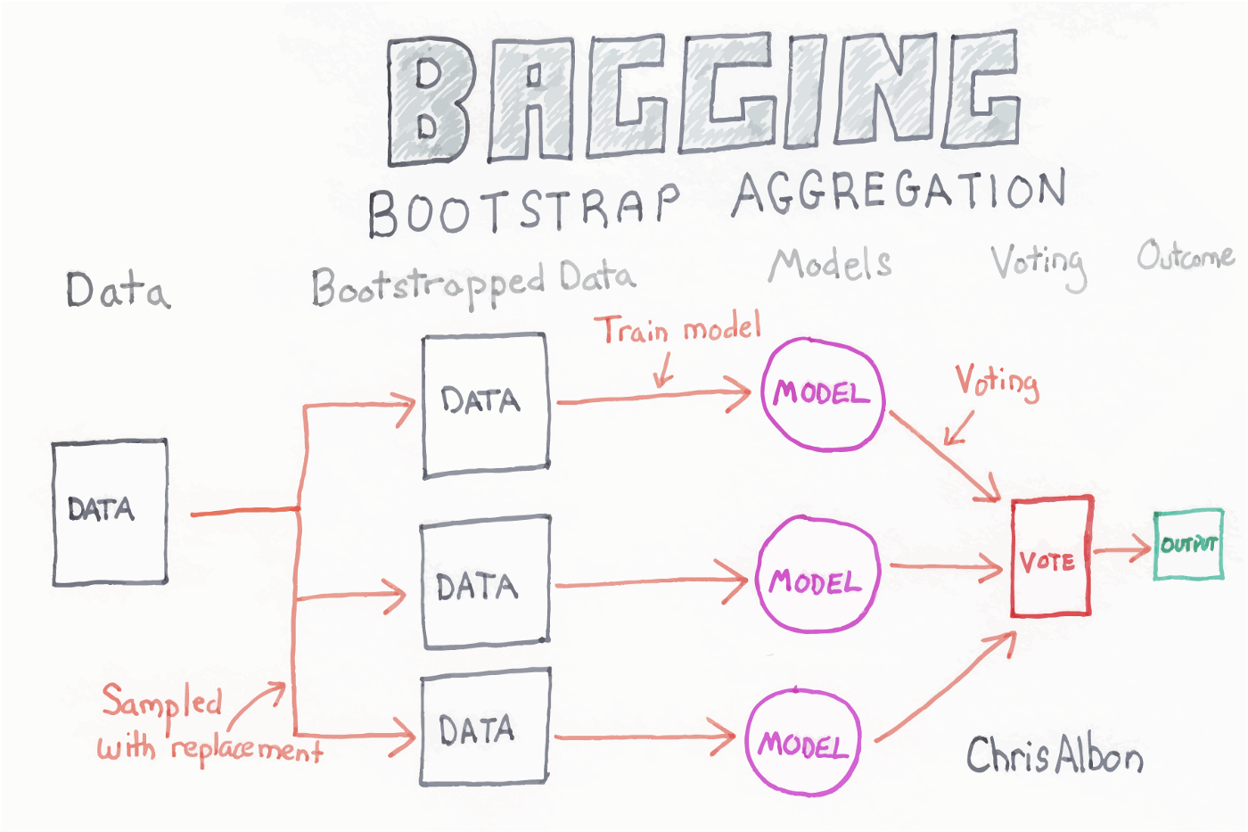
• Random Forest is an ensemble model that makes many decision trees using bagging, then takes a simple vote across them to assign a class
• XGBoost is another ensemble and arguably the most widely used (and useful) algorithm in tabular ML (it can do regression, classification, and julienne fries!)

• Deep Learning uses artificial neural networks with multiple layers to learn complex patterns from data. These models have performed well in a variety of tasks: image recognition, speech recognition, and natural language processing.

  Deep Learning models may also be used in unsupervised settings

Reference Card: train_test_split

• Function: sklearn.model_selection.train_test_split()
• Purpose: Split arrays or matrices into random train and test subsets.
• Key Parameters:
• *arrays: (Required) Sequence of indexables with same length / shape[0]. Allowed inputs are lists, numpy arrays, scipy-sparse matrices or pandas dataframes.
• test_size: (Optional, default=0.25) If float, should be between 0.0 and 1.0 and represent the proportion of the dataset to include in the test split. If int, represents the absolute number of test samples.
• train_size: (Optional, default=None) If float/int, represents the proportion/absolute number for the train split. If None, it's set to the complement of test_size.
• random_state: (Optional, default=None) Controls the shuffling applied to the data before applying the split. Pass an int for reproducible output across multiple function calls.
• shuffle: (Optional, default=True) Whether or not to shuffle the data before splitting.
• stratify: (Optional, default=None) If not None, data is split in a stratified fashion, using this as the class labels. Essential for imbalanced classification tasks.

Example:

from sklearn.model_selection import train_test_split
import numpy as np
X = np.array([[1, 2], [2, 3], [3, 4], [4, 5], [5, 6], [6, 7]])
y = np.array([0, 1, 0, 1, 0, 1])
# Split data: 70% train, 30% test, stratified by y, reproducible
X_train, X_test, y_train, y_test = train_test_split(
    X, y, test_size=0.3, random_state=42, stratify=y
)
print("X_train shape:", X_train.shape)
print("X_test shape:", X_test.shape)

🧠 Comprehension Checkpoint:

• What is the difference between supervised and unsupervised learning?
• Why do we split data into train and test sets?

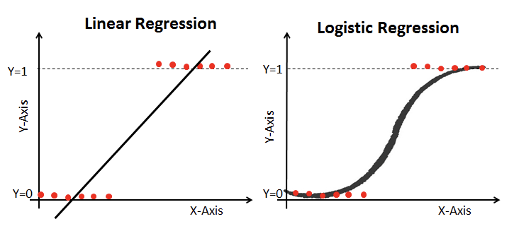
Logistic regression¶

Logistic regression works similarly to linear regression but uses a sigmoid curve that squeezes our straight line into an S-curve.

Reference Card: LogisticRegression

• Function: sklearn.linear_model.LogisticRegression()
• Purpose: Linear model for classification (binary or multinomial).
• Key Parameters:
• penalty: (Optional, default='l2') Specify the norm used in the penalization ('l1', 'l2', 'elasticnet', 'none').
• C: (Optional, default=1.0) Inverse of regularization strength; must be a positive float. Smaller values specify stronger regularization.
• solver: (Optional, default='lbfgs') Algorithm to use in the optimization problem. Common choices: 'liblinear' (good for small datasets), 'lbfgs', 'sag', 'saga' (faster for large ones).
• max_iter: (Optional, default=100) Maximum number of iterations taken for the solvers to converge.
• random_state: (Optional, default=None) Used when solver == ‘sag’, ‘saga’ or ‘liblinear’ to shuffle the data.

Example:

from sklearn.linear_model import LogisticRegression
X = [[1, 2], [2, 3], [3, 4]]
y = [0, 1, 0]
model = LogisticRegression().fit(X, y)
print(model.predict([[2, 2]]))

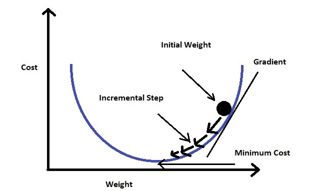
Additionally, it uses log loss in place of our usual mean-squared error cost function. This provides a convex curve for approximating variable weights using gradient descent.

• Logistic regression (interpretable ml)
• Logistic Regression using Gradient descent (kaggle)

Random forest¶

Each of the steps can be tweaked, but the general flow goes:

1. Bagging - create k random samples from the data set
2. Grow trees - individual decision trees are constructed by choosing the best features and cutpoints to separate the classes
3. Classify - instances are run through all trees and assigned a class by majority vote

Reference Card: RandomForestClassifier

• Function: sklearn.ensemble.RandomForestClassifier()
• Purpose: Ensemble of decision trees for classification
• Key Parameters:
• n_estimators: (Optional, default=100) The number of trees in the forest.
• max_depth: (Optional, default=None) The maximum depth of the tree. If None, then nodes are expanded until all leaves are pure or until all leaves contain less than min_samples_split samples.
• min_samples_split: (Optional, default=2) The minimum number of samples required to split an internal node.
• min_samples_leaf: (Optional, default=1) The minimum number of samples required to be at a leaf node.
• max_features: (Optional, default='sqrt') The number of features to consider when looking for the best split.

Boosted trees and gradient boosting¶

XGBoost¶

XGBoost stands for Extreme Gradient Boosting. Like other tree algorithms, XGBoost considers each instance with a series of if statements, resulting in a leaf with associated class assignment scores. Where XGBoost differs is that it uses gradient boosting to focus on weak-performing areas of the previous tree.

Reference Card: XGBClassifier

• Function: xgboost.XGBClassifier()
• Purpose: Implementation of the gradient boosting algorithm for classification.
• Key Parameters:
• n_estimators: (Optional, default=100) Number of gradient boosted trees. Equivalent to number of boosting rounds.
• learning_rate: (Optional, default=0.3) Boosting learning rate (xgb's "eta"). Step size shrinkage used in update to prevents overfitting.
• max_depth: (Optional, default=6) Maximum depth of a tree. Increasing this value will make the model more complex and more likely to overfit.
• subsample: (Optional, default=1.0) Subsample ratio of the training instance. Setting it to 0.5 means that XGBoost would randomly sample half of the training data prior to growing trees.
• colsample_bytree: (Optional, default=1.0) Subsample ratio of columns when constructing each tree.
• gamma: (Optional, default=0) Minimum loss reduction required to make a further partition on a leaf node of the tree.
• random_state: (Optional, default=None) Random number seed.

Example:

import xgboost as xgb
X = [[1, 2], [2, 3], [3, 4], [4, 5]]
y = [0, 1, 0, 1]
model = xgb.XGBClassifier(n_estimators=10).fit(X, y)
print(model.predict([[2, 2]]))

Boosted trees and gradient boosting¶

• Boosting - sequentially choosing models by minimizing errors from previous models while increasing the influence of high-performing models; i.e., each model tries to improve where the last was wrong
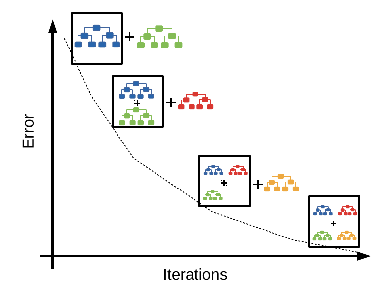
• Gradient boosting - a stagewise additive algorithm sequentially adding trees to improve performance measured by a loss function until some threshold is met. It's a greedy algorithm prone to overfitting but often proves useful when focused on poor-performing areas

Gradient Boosting Explained¶

Gradient Boosting is an iterative machine learning algorithm that is used to improve the accuracy of a model over time. Gradient Boosting works by building decision trees one at a time, where each subsequent tree is built to correct the errors of the previous tree.

How Gradient Boosting Works (Step-by-Step): 1. Start with a simple model: Build an initial decision tree on the training data. 2. Calculate errors: Compare the predictions of the tree to the actual values and calculate the errors (residuals). 3. Build a new tree for the errors: Train a new decision tree to predict the errors made by the previous tree, not the original target. 4. Update predictions: Add the new tree’s predictions to the previous predictions to get improved results. 5. Repeat: Continue building new trees, each time focusing on the remaining errors, until you reach a set number of trees or the model stops improving. 6. Combine all trees: The final prediction is a combination (sum) of all the trees’ outputs. 7. Minimize loss: The process uses gradient descent to minimize a loss function, making the model better at each step. 8. Result: The final model is highly accurate and can handle complex patterns, but care must be taken to avoid overfitting.

• XGBoost vs Random Forest (geek culture)
• Interpretable machine learning with XGBoost (towardsdatascience)

🧠 Comprehension Checkpoint:

• What is the main difference between random forest and XGBoost?
• Why might boosting lead to overfitting if not tuned carefully?

Deep learning¶

Conceptual Overview: Deep learning is a type of machine learning that uses networks of "neurons" (like a simplified brain) to learn from data. These models can learn very complex patterns, especially in images, text, and signals.

An example from TensorFlow Keras:

Reference Card: Keras Sequential Model

• Function: tensorflow.keras.Sequential() / tensorflow.keras.layers.Dense() / model.compile()
• Purpose: Build, configure, and prepare a linear stack of neural network layers for training.
• Key Parameters:
• layers.Dense(units): (Required) Number of neurons in the layer.
• layers.Dense(activation): (Optional) Activation function ('relu', 'sigmoid', 'softmax', etc.).
• layers.Dense(input_shape): (Required for first layer) Shape of the input data (tuple).
• model.compile(optimizer): (Required) Optimizer algorithm ('adam', 'sgd', etc.).
• model.compile(loss): (Required) Loss function ('binary_crossentropy', 'categorical_crossentropy', 'mse', etc.).
• model.compile(metrics): (Optional) List of metrics to evaluate during training (e.g., ['accuracy']).

Example:

from tensorflow import keras
from tensorflow.keras import layers
model = keras.Sequential([
    layers.Dense(8, activation='relu', input_shape=(2,)),
    layers.Dense(1, activation='sigmoid')
])
model.compile(optimizer='adam', loss='binary_crossentropy')
# model.fit(X_train, y_train, epochs=10)  # Uncomment to train

Deep learning is a subfield of machine learning that uses artificial neural networks with multiple layers to learn complex patterns from data. These models use back-propagation to adjust the weights in each layer during training, allowing them to model very large and complex datasets.

Deep learning models are especially useful for handling large datasets with high dimensionality, and they can be used for both supervised and unsupervised learning tasks. However, they often require a large amount of data and computation power to train effectively.

These models have performed well in a variety of tasks such as image recognition, speech recognition, and natural language processing.

• Artificial neural networks - a computational model inspired by biological neural networks that learn by adjusting the weights between neurons through training data
• Deep neural networks - an artificial neural network with more than one hidden layer; these additional layers enable the model to learn more complex patterns from the input data
• Convolutional neural networks - a type of deep neural network designed for image and video recognition tasks that use convolutional layers to detect features in the input data
• Recurrent neural networks - a type of deep neural network designed for sequence data that uses recurrent connections to remember previous inputs and outputs
• Popular frameworks - TensorFlow, PyTorch, and Keras are commonly used deep learning frameworks for building and training deep learning models. Each framework maintains a list of tutorials/examples for getting started (and plenty more on the web + youtube):
  • Keras
    • https://keras.io/getting_started/
    • Deep Learning with Python (free pdf)
  • Pytorch
    • https://pytorch.org/tutorials/
    • https://github.com/ritchieng/the-incredible-pytorch
  • Tensorflow
    • https://www.tensorflow.org/tutorials/quickstart/beginner
    • Tensorflow https://github.com/tensorflow/examples
  • JAX
    • https://jax.readthedocs.io/en/latest/notebooks/quickstart.html
    • https://github.com/gordicaleksa/get-started-with-JAX

Unsupervised models¶

Conceptual Overview: Unsupervised learning is about discovering hidden patterns or groupings in data when you don't know the "right answer" for each example.

Reference Card: Unsupervised Learning Methods

• Clustering: Group similar data points (e.g., K-means, hierarchical)
• Association: Find rules about how variables relate (e.g., Apriori)
• Dimensionality reduction: Reduce number of features (e.g., PCA, t-SNE)

Reference Card: KMeans

• Function: sklearn.cluster.KMeans()
• Purpose: Find groups (clusters) of similar data points in unlabeled data.
• Key Parameters:
• n_clusters: (Required) The number of clusters to form as well as the number of centroids to generate.
• init: (Optional, default='k-means++') Method for initialization ('k-means++', 'random'). 'k-means++' selects initial cluster centers in a smart way to speed up convergence.
• n_init: (Optional, default=10) Number of time the k-means algorithm will be run with different centroid seeds. The final results will be the best output of n_init consecutive runs in terms of inertia.
• max_iter: (Optional, default=300) Maximum number of iterations of the k-means algorithm for a single run.
• random_state: (Optional, default=None) Determines random number generation for centroid initialization. Use an int to make the randomness deterministic.

Example:

from sklearn.cluster import KMeans
import numpy as np
X = np.array([[1, 2], [1.5, 1.8], [5, 8], [8, 8], [1, 0.6], [9, 11]])
kmeans = KMeans(n_clusters=2, random_state=42, n_init='auto').fit(X)
print("Cluster labels:", kmeans.labels_)
print("Cluster centers:", kmeans.cluster_centers_)

• Clustering: grouping points based on similarities/differences; e.g., proximity and separability of data, market segmentation, image compression
  • K-means (and Fuzzy K-means)
  • Hierarchical clustering (e.g., BIRCH)
  • Gaussian mixture
  • Affinity Propagation
  • Anomaly detection
    • Isolation Forest
    • Local Outlier Factor
    • Min Covariant Determinant
• Association: reveals relationships between variables; e.g., A goes up and B goes down, people who buy X also buy Y
  • Apriori
  • Equivalence Class Transformation (eclat)
  • Frequent-Pattern (F-P) Growth
• Dimensionality reduction: reduces the inputs to a smaller size while attempting to preserve predictive power; e.g., removing noise and collinearity
  • Principal Component Analysis
  • Manifold Learning — LLE, Isomap, t-SNE
  • Autoencoders

Links to learn more:

• Unsupervised Learning: Algorithms and Examples (altexsoft)

📉 How models fail¶

Conceptual Overview: Even the best models can fail if the data is messy, the problem is hard, or the world changes. Common failure modes include:

• Bad or inconsistent labels (garbage in, garbage out!)
• Underfitting (model too simple) or overfitting (model too complex)
• Dataset shift (data changes between training and real-world use)
• Hidden confounders (Simpson's paradox)
• Imbalanced or "troublesome" classes

Labeling¶

Oh, labeling…

Labeling issues can arise when the data is not labeled correctly or consistently, which can lead to biased or inaccurate models. Examples of labeling issues include:

• Mislabeling: Labels that are assigned to data points are incorrect.
• Ambiguous labeling: Labels that are assigned to data points are not clear or specific.
• Inconsistent labeling: Labels that are assigned to similar data points are not the same

Fit¶

A model may fail to fit the data in one of two ways: under-fitting or over-fitting:

• Under-fitting: The model fails to capture the the differences between the classes. The model may be too simple, lack the necessary features, or the classes may not easily divide based on existing data.

• Over-fitting: The model fits the training data too closely, leading to poor generalization. This can be the case when the model is overly complex or the data may have "too many features".

  Note: With enough variables you can build a perfect predictor for anything (at least in the training set). That doesn't mean the model will perform well in the wild

Dataset Shift¶

Dataset shift occurs when the distribution of the data changes between the training and test sets. Dataset shift can be divided into three types:

1. Covariate Shift: A change in the distribution of the independent variables between the training and test sets.
2. Prior Probability Shift: A change in the distribution of the target variable between the training and test sets.
3. Conceptual Shift: A change in the relationship between the independent and target variables between the training and test sets.

See: https://d2l.ai/chapter_linear-classification/environment-and-distribution-shift.html

Simpson's Paradox¶

Simpson's paradox occurs when a trend appears in several different groups of data, but disappears or reverses when these groups are combined. It is a common problem in statistics and machine learning that can occur when there are confounding variables that affect the relationship between the independent and dependent variables.

Troublesome classes¶

Certain classes or categories in a dataset may be more difficult to classify accurately than others. This can be due to imbalanced class distribution, noisy data, or other factors. Identifying and addressing troublesome classes is an important step in building effective classification models.

Additional topics that could be added to this section include:

• Bias and fairness in classification models
• Lack of interpretability in black-box models
• Adversarial attacks and robustness of classification models
• Transfer learning and domain adaptation in classification models
• Active learning and semi-supervised learning for classification.

🧠 Comprehension Checkpoint:

• What is overfitting, and why is it a problem?
• Give an example of how dataset shift could affect a health prediction model.
• Why is it important to check for labeling errors in your data?

🚀 Automated Feature Engineering¶

Automated feature engineering is the process of using algorithms or libraries to automatically create new features from your existing data—without having to manually invent each one. Instead of hand-coding every transformation, automated tools systematically combine, aggregate, and transform your raw variables to generate a much larger set of potentially useful features.

• Why automate?

  • Saves time and reduces manual effort, especially with large or complex datasets.
  • Can discover subtle or non-obvious patterns by combining features in ways a human might not think of.
  • Especially powerful for relational data (multiple linked tables) and time series, where relationships and trends can be hard to spot.

• How does it work?

  • Automated feature engineering tools apply a set of mathematical operations (like sum, mean, count, difference, ratio, etc.) to your data, often stacking these operations across different columns or tables.
  • For example, you might automatically generate features like "average blood pressure per patient," "number of visits in the last month," or "maximum heart rate difference between visits."

🛠️ Featuretools Library: Automated Feature Synthesis¶

Featuretools is a Python library that automates the creation of new features from your data, especially when you have multiple related tables (like patients, visits, and labs). Its core innovation is deep feature synthesis (DFS), which systematically combines and stacks simple operations—like sum, mean, count, difference, and ratios—across different variables and tables to generate complex, multi-level features.

• What is Deep Feature Synthesis (DFS)?

  • DFS works by chaining together basic operations (called "primitives") to create new features. For example, it might:
    • Aggregate: Compute the mean, sum, or count of lab results for each patient.
    • Transform: Calculate the difference between a patient's max and min blood pressure.
    • Combine: Stack these operations, such as "mean of the difference in lab values per visit per patient."
  • DFS explores many possible combinations, including across relationships (e.g., "number of visits in last 30 days" or "average glucose per visit per patient").

• Why is this useful in health data?

  • Health records are often spread across multiple tables (patients, visits, labs, medications).
  • DFS can automatically create features that summarize a patient's history, recent trends, or event counts—without you having to write custom code for each one.
  • This approach can reveal subtle patterns and relationships that manual feature engineering might miss.

Reference Card: featuretools.dfs

• Function: featuretools.dfs() (Deep Feature Synthesis)
• Purpose: Automatically generate features from relational datasets organized in an EntitySet.
• Key Parameters:
• entityset: (Required) A Featuretools EntitySet object containing dataframes and their relationships.
• target_dataframe_name: (Required) The name of the dataframe for which to build features.
• agg_primitives: (Optional) List of aggregation primitives (e.g., 'mean', 'sum', 'count', 'std') to apply across relationships.
• trans_primitives: (Optional) List of transformation primitives (e.g., 'month', 'weekday', 'diff', 'percentile') to apply to single columns.
• max_depth: (Optional, default=2) Maximum depth of features to create (how many primitives to stack).
• features_only: (Optional, default=False) If True, return only the list of feature definitions instead of computing the feature matrix.

Example:

import featuretools as ft
import pandas as pd

# Example: patients and visits
patients = pd.DataFrame({'patient_id': [1, 2], 'age': [65, 70]})
visits = pd.DataFrame({'visit_id': [1, 2, 3], 'patient_id': [1, 1, 2], 'bp': [120, 130, 125]})

es = ft.EntitySet(id='health')
es = es.add_dataframe(dataframe_name='patients', dataframe=patients, index='patient_id')
es = es.add_dataframe(dataframe_name='visits', dataframe=visits, index='visit_id')
es = es.add_relationship('patients', 'patient_id', 'visits', 'patient_id')

feature_matrix, feature_defs = ft.dfs(entityset=es, target_dataframe_name='patients')
print(feature_matrix)

<!---
This code demonstrates Deep Feature Synthesis (DFS) using Featuretools. First, an `EntitySet` is created to define the tables (`patients`, `visits`) and their relationship. Then, `ft.dfs` automatically generates features for the `target_dataframe_name` ('patients') by applying aggregation primitives (like MEAN, COUNT of visits' 'bp') and transformation primitives. This automates the creation of potentially hundreds of features, saving significant effort, especially with complex relational health data. Beginners might find setting up the EntitySet relationships the trickiest part.
--->

### 🩺 Domain-Specific Feature Derivations

Sometimes, the best features come from domain knowledge—knowing what matters in health data.

- **Examples:**
    - Calculating BMI from height and weight
    - Deriving heart rate variability from RR intervals
    - Creating a "polypharmacy" flag for patients on multiple medications

#### Example: Creating a BMI feature

```python
import pandas as pd

df = pd.DataFrame({'weight_kg': [70, 80], 'height_m': [1.75, 1.80]})
df['BMI'] = df['weight_kg'] / (df['height_m'] ** 2)
print(df)

Model Interpretation with Tree-Based Models¶

Understanding why a model makes its predictions is crucial in health data science—especially when decisions impact patient care. Tree-based models (like Random Forests and XGBoost) can be interpreted using specialized tools that reveal which features drive predictions.

SHAP Values for Feature Importance¶

SHAP (SHapley Additive exPlanations) assigns each feature an importance value for a particular prediction, based on cooperative game theory.

Reference Card: shap.TreeExplainer & shap.summary_plot

• Function: shap.TreeExplainer(model), shap.summary_plot(shap_values, features)
• Purpose: Explain the output of tree-based models (like XGBoost, RandomForest) using SHAP values. summary_plot visualizes global feature importance.
• Key Parameters:
• TreeExplainer(model): (Required) The tree-based model object to explain.
• TreeExplainer(data): (Optional) A background dataset used for conditioning (often the training data).
• explainer.shap_values(X): (Required) The data instances (e.g., test set) for which to compute SHAP values.
• summary_plot(shap_values): (Required) The computed SHAP values.
• summary_plot(features): (Required) The feature data corresponding to shap_values.
• summary_plot(plot_type): (Optional, default="dot") Type of plot ('dot', 'bar', 'violin').

Example:

import shap
import xgboost as xgb
import pandas as pd

# Train a simple model (example)
X = pd.DataFrame({'age': [50, 60], 'bp': [120, 140]})
y = [0, 1]
model = xgb.XGBClassifier().fit(X, y)

# Explain predictions
explainer = shap.TreeExplainer(model)
shap_values = explainer.shap_values(X)

Visualize feature importance¶

shap.summary_plot(shap_values, X, plot_type="bar")

Example SHAP summary plot: Each dot shows a feature's impact on a prediction. Color indicates feature value (red=high, blue=low).

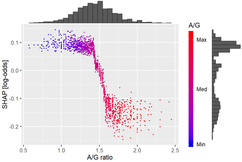Example SHAP dependence plot: Shows how the effect of one feature depends on the value of another feature. In this case the A/G ratio (albumin to globulin in blood) has a cutoff ~1.5 for a change in prognosis.

eli5 for Model Inspection¶

eli5 is a Python library that helps demystify machine learning models by showing feature weights and decision paths.

Reference Card: eli5.show_weights

• Function: eli5.show_weights()
• Purpose: Explain weights and feature importances of black-box or white-box estimators.
• Key Parameters:
• estimator: (Required) Trained scikit-learn compatible estimator object.
• feature_names: (Optional) List of feature names corresponding to the columns in the input data.
• top: (Optional, default=None) Number of top features to show. If None, show all features.
• target_names: (Optional) Names for the target variable classes.

Example:

import eli5
from sklearn.ensemble import RandomForestClassifier

X = [[1, 2], [3, 4], [5, 6]]
y = [0, 1, 0]
model = RandomForestClassifier().fit(X, y)

# Show feature importances
eli5.show_weights(model, feature_names=['feature1', 'feature2'])

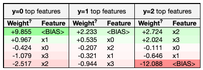Example eli5 feature importance visualization for a tree-based model.

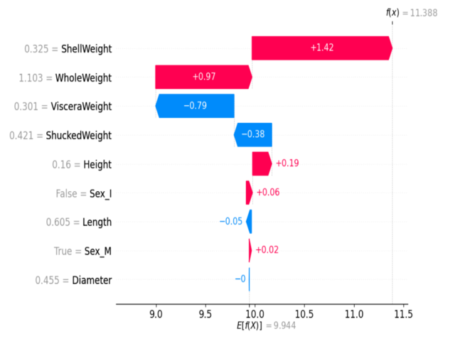
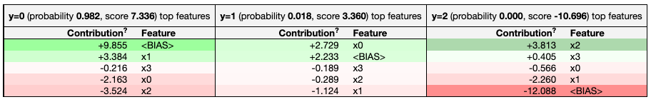Example eli5 explanation of a single prediction, showing how each feature contributed.

Example eli5 visual breakdown of a single prediction, highlighting the contribution of each feature.

Interpreting Feature Interactions¶

Tree-based models can capture interactions between features (e.g., age and blood pressure together may be more predictive than either alone). Tools like SHAP can help visualize these interactions.

Example: SHAP dependence plot¶

# Continuing from previous SHAP example
shap.dependence_plot('age', shap_values, X)

🧪 LIVE DEMO 2: Classification with Derived Features¶

A hands-on demo of feature engineering from time series sensor data, comparing RandomForest and XGBoost, and interpreting results with eli5 and SHAP. See: demo/02_basic_classification.md

Practical Data Preparation¶

Preparing your data is just as important as choosing the right model. Good data prep can make or break your results—especially with real-world health data, which is often messy, imbalanced, and full of categorical variables.

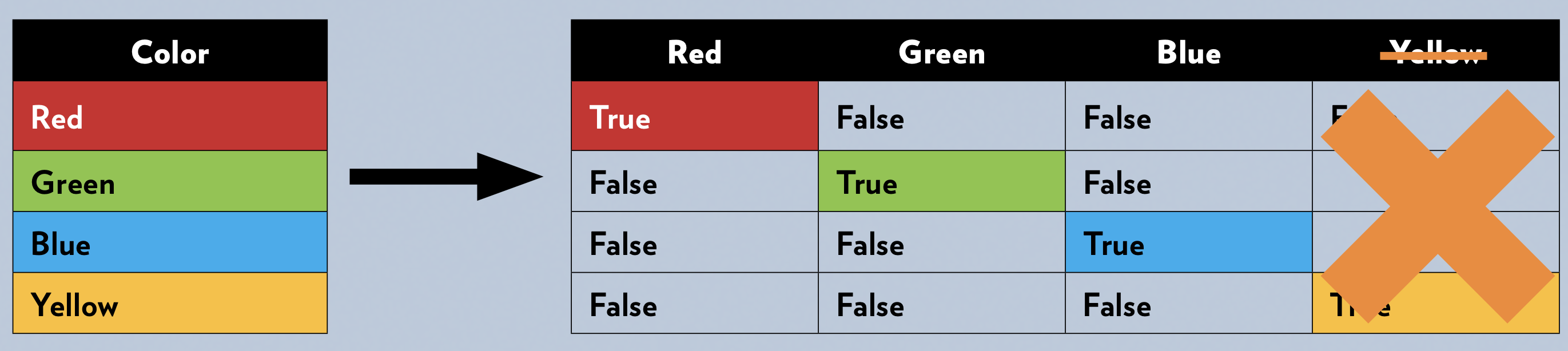
OneHotEncoder for Categorical Variables¶

Many machine learning models require all input features to be numeric. One-hot encoding transforms categorical variables (like "smoker" or "blood type") into a set of binary columns.

Reference Card: OneHotEncoder

• Function: sklearn.preprocessing.OneHotEncoder()
• Purpose: Encode categorical features as a one-hot numeric array.
• Key Parameters:
• categories: (Optional, default='auto') Categories per feature. 'auto' determines categories automatically from the training data.
• drop: (Optional, default=None) Specifies a category to drop for each feature ('first', 'if_binary', or an array). Helps avoid multicollinearity.
• sparse_output: (Optional, default=True) Will return sparse matrix if set True else will return an array. Changed from sparse in newer versions.
• handle_unknown: (Optional, default='error') Whether to raise an error or ignore if an unknown categorical feature is present during transform ('error', 'ignore', 'infrequent_if_exist').

Example:

from sklearn.preprocessing import OneHotEncoder
import pandas as pd

df = pd.DataFrame({'smoker': ['yes', 'no', 'no', 'yes']})
encoder = OneHotEncoder(sparse=False, handle_unknown='ignore')
encoded = encoder.fit_transform(df[['smoker']])
print(encoded)

<!---
This code uses `OneHotEncoder` to transform a categorical feature ('smoker') into numerical format suitable for most ML algorithms. Each category becomes a new binary column (0 or 1). Setting `sparse_output=False` (or `sparse=False` in older sklearn) returns a dense NumPy array, often easier for beginners. `handle_unknown='ignore'` is crucial for real-world data where the test set might contain categories not seen during training. Remember to fit the encoder *only* on the training data and then transform both train and test sets.
--->

![onehotencoder](media/onehotencoder.png)

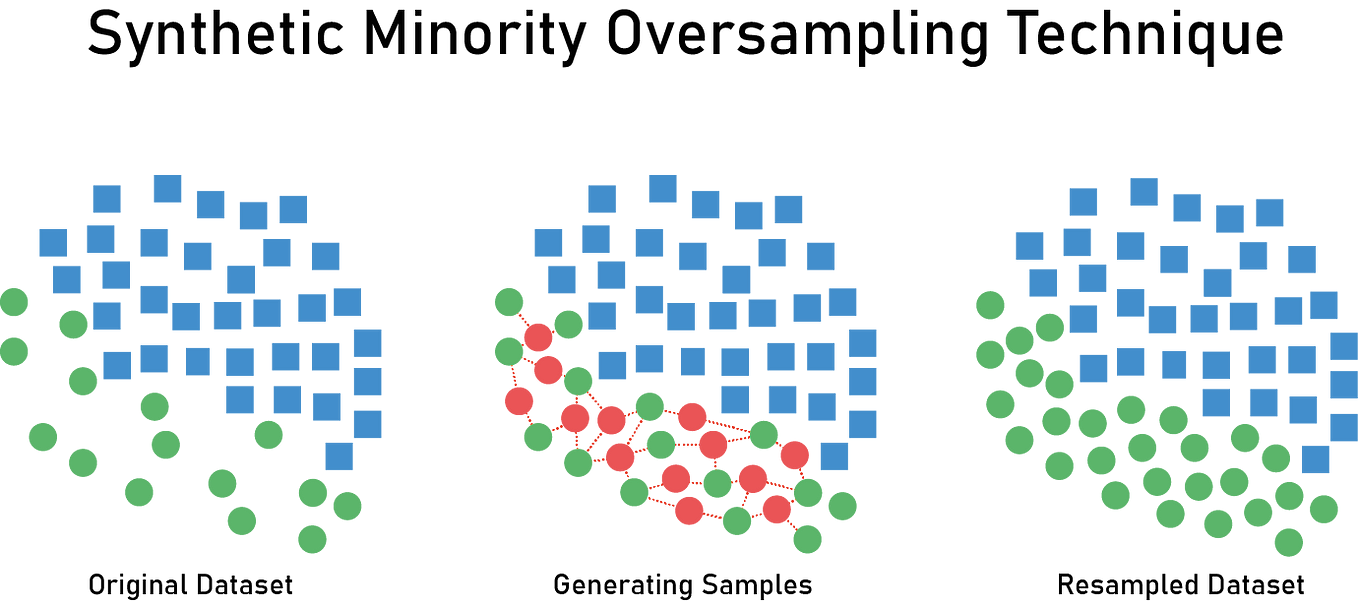
### Handling Imbalanced Data with SMOTE

In health data, one class (like "disease present") is often much rarer than the other. **SMOTE** (Synthetic Minority Over-sampling Technique) creates synthetic examples of the minority class to balance the dataset.

![smote](media/smote.png)

**Reference Card: `SMOTE`**

- **Function:** `imblearn.over_sampling.SMOTE()` (Synthetic Minority Over-sampling Technique)
- **Purpose:** Address class imbalance by oversampling the minority class(es) by creating synthetic samples.
- **Key Parameters:**
  - `sampling_strategy`: (Optional, default='auto') Specifies the target class distribution after resampling. 'auto' resamples all minority classes to match the majority class count. Can be a float (ratio relative to majority) or a dict `{class_label: count}`.
  - `k_neighbors`: (Optional, int, default=5) Number of nearest neighbors in the minority class used as a basis for generating synthetic samples.
  - `random_state`: (Optional, int, default=None) Controls the randomization of the algorithm for reproducible results.

**Example:**

```python
from imblearn.over_sampling import SMOTE
from sklearn.datasets import make_classification
import numpy as np
import collections # To display class counts

# Create a sample imbalanced dataset (e.g., 90 class 0, 10 class 1)
X, y = make_classification(n_samples=100, n_features=2, n_informative=2,
                           n_redundant=0, n_repeated=0, n_classes=2,
                           n_clusters_per_class=1, weights=[0.9, 0.1],
                           class_sep=0.8, random_state=42)

print("Original dataset shape %s" % collections.Counter(y))

# Apply SMOTE
smote = SMOTE(random_state=42)
X_resampled, y_resampled = smote.fit_resample(X, y)

print("Resampled dataset shape %s" % collections.Counter(y_resampled))
# print("Resampled X shape:", X_resampled.shape) # Uncomment to see shape

When and How to Combine Techniques¶

Often, you'll need to use several data prep techniques together: splitting, encoding, scaling, balancing, and more. The order is crucial to prevent data leakage and ensure reliable model evaluation!

• Recommended Order:
• Encode categorical variables: Fit the encoder only on the training data, then transform both the training and test data.
• Scale/normalize features (if needed): Fit the scaler only on the training data, then transform both the training and test data.
• Split into train/test sets: Isolate your test set completely. Consider using stratified sampling (stratify=y in train_test_split) to ensure both train and test sets have similar proportions of each class, especially important with imbalanced data.

• Balance classes (Optional, e.g., SMOTE): Apply balancing techniques only to the training set. Never apply balancing to the test set, as this would leak information and give an unrealistic performance estimate.

• Why this order?

  • Transform encoders and scalers on the data to ensure the train and test set have identical schemas for the model to use.
  • Splitting after transformation ensures consistent data representation across both training and test sets.
  • Balancing only the training set prevents the model from being evaluated on synthetic data and ensures the test set reflects the original class distribution (or the expected real-world distribution).

• If Not Balancing: If you choose not to balance the training data (e.g., due to concerns about introducing noise with synthetic data), it's crucial to use evaluation metrics that account for imbalance. Don't rely solely on accuracy. Instead, focus on:

  • Confusion Matrix: To see performance per class (TP, TN, FP, FN).
  • Precision, Recall, F1-score: Especially the F1-score, which balances precision and recall. Consider these metrics for the minority class specifically.
  • ROC AUC: While useful, remember it can be misleadingly high on imbalanced data. Consider Precision-Recall AUC as an alternative.

🧪 LIVE DEMO 3: Imbalanced Classification & Model Interpretation¶

A hands-on demo for handling imbalanced classes, categorical feature encoding, SMOTE, and model interpretation with eli5. See: demo/03_imbalanced_classification.md