Lecture 09: Data Visualization & Communication
-1. Project Inspiration
0. Introduction (5 minutes)
The Data Communication Crisis
Picture this: You've just completed a groundbreaking analysis showing that a simple intervention could reduce costs by 23%. You present a dense Excel table with 47 rows of statistics to the board. Eyes glaze over. Your brilliant insight dies in a spreadsheet graveyard. 💀
Now imagine instead: An interactive dashboard where stakeholders can explore the data themselves, see the intervention's impact across different segments, and watch the savings accumulate in real-time. Which presentation gets funding? 🎯
Lecture Objectives:
- Create clear process diagrams using Mermaid for workflows and data pipelines
- Build interactive visualizations with Altair that tell compelling data stories
- Generate automated, shareable reports using MkDocs for disseminating findings
- Develop professional dashboards with Dash by Plotly for data exploration
- Apply these tools to real-world scenarios, focusing on principles of effective communication
Agenda Overview:
graph TD
    A[Intro: The Power of Visual Communication] --> B(Diagramming: Mermaid);
    B --> C(Interactive Viz: Altair);
    C --> D(Automated Reports: MkDocs);
    D --> E(Dashboards: Dash by Plotly);
1. Diagrams as Code with Mermaid (15 minutes)
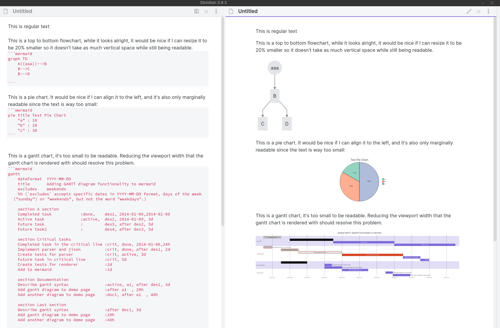
Visualizing processes, architectures, and workflows is essential for understanding and communicating complex systems. While many tools exist for creating diagrams, the "diagrams as code" approach offers unique advantages for data science projects.
1.1. Why Diagrams as Code?
- Concept: Treating diagrams as source code offers several advantages. These diagrams are defined using text, making them version-controllable with tools like Git, inherently reproducible, and easier to update systematically. <!---
- Instead of using a graphical user interface (GUI) to draw shapes and connectors, you write text-based definitions that a tool then renders into a visual diagram.
- This is particularly valuable where processes and workflows need to be clearly documented and updated. --->
- Benefits: This approach promotes:
- Consistency: Diagrams maintain a uniform style, especially across a team or project.
- Version Control: Changes to diagrams can be tracked, diffed, and reverted using Git, just like any other code. This is invaluable for collaborative projects and understanding the evolution of workflows.
- Reproducibility: Anyone with the text definition can regenerate the exact same diagram, ensuring consistent documentation.
- Easy Integration: Text-based diagrams can be easily embedded into documentation (like MkDocs sites), README files, or even code comments.
- Collaboration: Team members can collaborate on diagrams using familiar code review workflows.
- Accessibility: Text-based definitions can be more accessible to individuals using screen readers than complex image files, although the rendered output's accessibility also matters. <!---
- Reproducibility ensures that the diagram accurately reflects the documented workflow at any point in time.
- Ease of integration means diagrams live alongside the documentation or code they describe, reducing the chance of them becoming outdated or lost. --->
- Contrast with GUI Tools: GUI-based diagramming tools (e.g., Microsoft Visio, Lucidchart, draw.io) offer a visual interface for drawing. While often user-friendly for initial creation, they can be challenging for:
- Versioning: Tracking precise changes can be difficult, which is crucial for workflow documentation.
- Reproducibility: Ensuring identical regeneration by different users or on different systems can be tricky.
- Programmatic Updates: Making systematic changes across many diagrams is often manual.
- Integration with Code/Docs: Often involves exporting static images, which can become outdated. <!---
- GUI tools excel at free-form drawing and quick mockups.
- "Diagrams as code" tools shine when diagrams need to be maintained, versioned, and integrated with technical documentation over time. --->
1.2. Introduction to Mermaid
Mermaid is a popular JavaScript-based tool that takes Markdown-inspired text definitions and renders them as diagrams. It's designed to be simple to learn yet powerful enough for a variety of diagramming needs.
- What is Mermaid? Mermaid is a JavaScript-based diagramming and charting tool that uses Markdown-inspired text definitions to dynamically create and modify diagrams. You write text, Mermaid draws the picture. <!---
- The "Markdown-inspired" part means its syntax is generally human-readable and relatively simple, much like Markdown for text formatting. --->
- Common Diagram Types: It supports various diagram types, including:
- Flowcharts: For visualizing processes, workflows, and decision trees. (e.g.,
graph TD; A-->B;)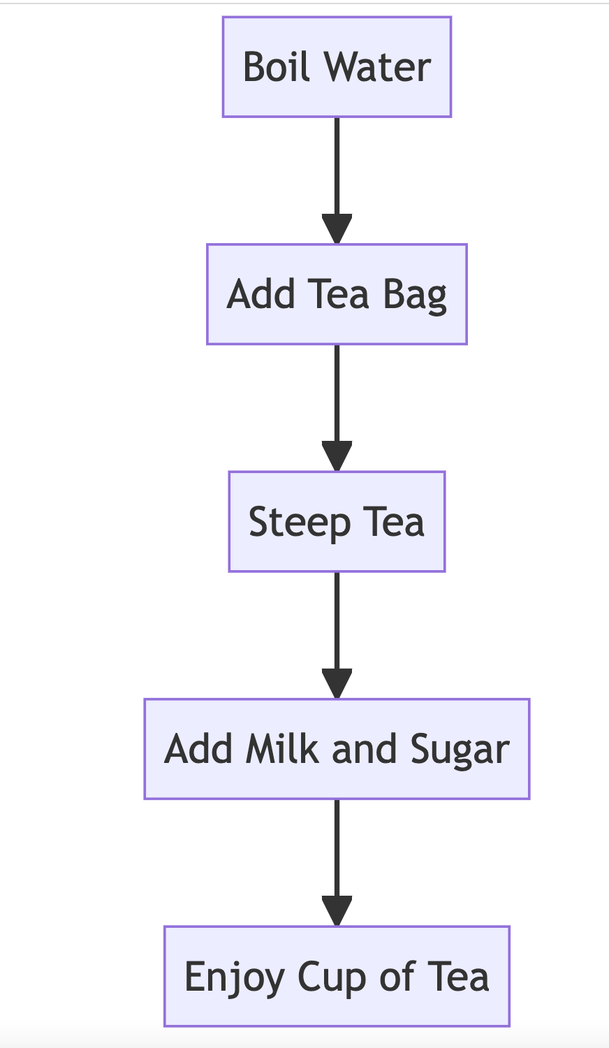
- Sequence Diagrams: For showing interactions between different components or actors over time. (e.g.,
sequenceDiagram; User->>System: Submit Request;)
- Gantt Charts: For project scheduling and tracking timelines.
- Class Diagrams: For visualizing software structures.
- Entity Relationship Diagrams (ERDs): For database schema design.
- And more (User Journey, Process Flow, System Design, etc.). <!---
- Flowcharts and sequence diagrams are particularly useful for documenting workflows, user pathways, or system interactions. --->
- Flowcharts: For visualizing processes, workflows, and decision trees. (e.g.,
- Tools for Mermaid:
- Online Editor: The Mermaid Live Editor is an excellent resource for quickly writing, previewing, and sharing Mermaid diagrams.
- VS Code Extensions: Many extensions provide live preview capabilities for Mermaid diagrams within Markdown files (e.g., "Markdown Preview Mermaid Support," "Mermaid Markdown Syntax Highlighting").
- MkDocs Integration: Many MkDocs themes (like Material for MkDocs) have built-in support for Mermaid, or it can be added via plugins. We'll see this later.
- Other Platforms: GitHub, GitLab, and some other platforms also render Mermaid diagrams directly in Markdown files. <!---
- The Mermaid Live Editor (mermaid.live) is a convenient online resource for quickly drafting and testing Mermaid diagrams.
- Native rendering support in platforms like GitHub and GitLab makes it easy to include diagrams directly in project READMEs or wikis. --->
1.3. Basic Mermaid Syntax & Examples
Let's focus on flowcharts, as they are broadly applicable to many workflows.
Flowcharts
Flowcharts are used to represent processes, workflows, or algorithms, showing steps as boxes of various kinds, and their order by connecting them with arrows.
- Concept: Visualizing processes, step-by-step logic, and decision points.
- Reference Card: Mermaid Flowchart
- Declaration: Start with
graph TD;(for Top-Down) orgraph LR;(for Left-Right). Other orientations likeBT(Bottom-Top) andRL(Right-Left) also exist. <!---TDorTBfor Top to Bottom.LRfor Left to Right. --->
- Nodes (Shapes):
id[Text]Default rectangle:A[Data Collection]id(Text)Rounded rectangle:B(Data Processing)id((Text))Circle:C((Analysis))id{Text}Diamond (for decisions):D{Results Significant?}id>Text]Asymmetric/Stadium:E>Report Generation]- Many other shapes are available (parallelogram, trapezoid, etc.). <!---
- The
idis a unique identifier for the node, used for linking. TheTextis what's displayed. - Choosing the right shape can help convey the meaning of a step (e.g., diamond for decisions). --->
- Links (Connections):
A --> B(Arrow link from A to B)A --- B(Line link from A to B)A -- Text --> B(Arrow link with text on the arrow)A -.-> B(Dotted arrow link)A == Text ==> B(Thick arrow link with text) <!---- Links define the flow and relationships between steps.
- Text on links can clarify conditions or actions. --->
- Declaration: Start with
-
Minimal Example (Data Analysis Pipeline): This diagram outlines a typical workflow for a data analysis project.
graph TD;
    A[Load Data] --> B(Data Cleaning & Preprocessing);
    B --> C{Select Analysis Type};
    C -- Descriptive Stats --> D[Generate Summary];
    C -- Predictive Model --> E[Train & Evaluate Model];
    D --> F[Visualize Key Metrics];
    E --> F;
    F --> G[Compile Report];
graph TD; A[Load Data] --> B(Data Cleaning & Preprocessing); B --> C{Select Analysis Type}; C -- Descriptive Stats --> D[Generate Summary]; C -- Predictive Model --> E[Train & Evaluate Model]; D --> F[Visualize Key Metrics]; E --> F; F --> G[Compile Report];
More Workflow Examples
Decision Support System:
graph TD;
A[User Input] --> B{Risk Assessment};
B -->|High Risk| C[Immediate Alert];
B -->|Medium Risk| D[Schedule Review];
B -->|Low Risk| E[Standard Processing];
C --> F[Emergency Protocol];
D --> G[Follow-up Planning];
E --> H[Regular Processing];
graph TD;
A[User Input] --> B{Risk Assessment};
B -->|High Risk| C[Immediate Alert];
B -->|Medium Risk| D[Schedule Review];
B -->|Low Risk| E[Standard Processing];
C --> F[Emergency Protocol];
D --> G[Follow-up Planning];
E --> H[Regular Processing];User Journey Through System:
graph LR;
A[User Entry] --> B{Initial Check};
B -->|Critical| C[Priority Processing];
B -->|Standard| D[Regular Queue];
B -->|Basic| E[Simple Processing];
C --> F[Main Process];
D --> F;
E --> F;
F --> G{Outcome};
G -->|Success| H[Complete];
G -->|Needs Review| I[Review Process];
G -->|Error| J[Error Handling];
graph LR;
A[User Entry] --> B{Initial Check};
B -->|Critical| C[Priority Processing];
B -->|Standard| D[Regular Queue];
B -->|Basic| E[Simple Processing];
C --> F[Main Process];
D --> F;
E --> F;
F --> G{Outcome};
G -->|Success| H[Complete];
G -->|Needs Review| I[Review Process];
G -->|Error| J[Error Handling];Demo 1: Mermaid Flowchart
- (Refer to
lectures/09/demo/01_mermaid_flowchart.md) <!---- The first demo will provide hands-on practice with creating a simple flowchart.
- Students will apply the syntax learned to visualize a familiar process. --->
1.4. More Mermaid Examples
Here are some practical examples showing different node shapes and their use cases in healthcare workflows. Each example shows both the code and the rendered diagram:
Clinical Trial Enrollment Flow
Reference Card: Mermaid Flowchart - Declaration: graph TD; (Top-Down) or graph LR; (Left-Right) - Node Types: - [()] - Database/Storage - () - Process/Step - {} - Decision Point - [[]] - Subroutine/Complex Process - >] - Output/Document - (()) - End Point/Result - Links: - --> - Arrow link - -- Text --> - Labeled arrow - -.-> - Dotted arrow
Code:
graph TD;
A[(Patient Database)] --> B{Meets Criteria?};
B -->|Yes| C[Screen Patient];
B -->|No| D[Document Exclusion];
C --> E{Consent Given?};
E -->|Yes| F[[Randomization]];
E -->|No| G[Document Refusal];
F --> H[Intervention Group];
F --> I[Control Group];
H --> J>Follow-up Visits];
I --> J;
J --> K((Study End));
graph TD;
A[(Patient Database)] --> B{Meets Criteria?};
B -->|Yes| C[Screen Patient];
B -->|No| D[Document Exclusion];
C --> E{Consent Given?};
E -->|Yes| F[[Randomization]];
E -->|No| G[Document Refusal];
F --> H[Intervention Group];
F --> I[Control Group];
H --> J>Follow-up Visits];
I --> J;
J --> K((Study End));Hospital Admission Process
Code:
graph LR;
A[Patient Arrival] --> B{Urgency Level};
B -->|Emergency| C[[ER Triage]];
B -->|Scheduled| D[Registration];
C --> E{Stable?};
E -->|Yes| D;
E -->|No| F[Immediate Care];
D --> G[Room Assignment];
F --> G;
G --> H>Treatment Plan];
graph LR;
A[Patient Arrival] --> B{Urgency Level};
B -->|Emergency| C[[ER Triage]];
B -->|Scheduled| D[Registration];
C --> E{Stable?};
E -->|Yes| D;
E -->|No| F[Immediate Care];
D --> G[Room Assignment];
F --> G;
G --> H>Treatment Plan];Data Pipeline with Error Handling
Code:
graph TD;
A[(Raw Data)] --> B[Validation];
B --> C{Valid?};
C -->|Yes| D[Processing];
C -->|No| E>Error Log];
E --> F[Manual Review];
F -->|Fixed| B;
F -->|Unfixable| G[[Archive]];
D --> H[Analysis];
H --> I((Results));
graph TD;
A[(Raw Data)] --> B[Validation];
B --> C{Valid?};
C -->|Yes| D[Processing];
C -->|No| E>Error Log];
E --> F[Manual Review];
F -->|Fixed| B;
F -->|Unfixable| G[[Archive]];
D --> H[Analysis];
H --> I((Results));1.5. Mermaid Configuration
Mermaid supports various configuration options to customize the appearance of diagrams. Here are some key configurations:
-
Theme: You can switch between different themes (e.g., default, dark, forest) using the
%%{init: {'theme': 'theme_name'}}%%directive.%%{init: {'theme': 'dark'}}%% graph TD; A[Load Data] --> B(Data Cleaning & Preprocessing); B --> C{Select Analysis Type}; C -- Descriptive Stats --> D[Generate Summary]; C -- Predictive Model --> E[Train & Evaluate Model]; D --> F[Visualize Key Metrics]; E --> F; F --> G[Compile Report];%%{init: {'theme': 'dark'}}%% graph TD; A[Load Data] --> B(Data Cleaning & Preprocessing); B --> C{Select Analysis Type}; C -- Descriptive Stats --> D[Generate Summary]; C -- Predictive Model --> E[Train & Evaluate Model]; D --> F[Visualize Key Metrics]; E --> F; F --> G[Compile Report]; -
Style: You can apply custom styles to nodes, links, and overall diagram appearance using the
%%{init: {'themeVariables': {...}}}%%directive.%%{init: {'themeVariables': { 'fontSize': '16px', 'fontFamily': 'Arial', 'primaryColor': '#ff0000', 'primaryTextColor': '#fff', 'primaryBorderColor': '#7C0000', 'lineColor': '#F8B229', 'secondaryColor': '#006100', 'tertiaryColor': '#fff' }}}%% graph TD; A[Load Data] --> B(Data Cleaning & Preprocessing); B --> C{Select Analysis Type}; C -- Descriptive Stats --> D[Generate Summary]; C -- Predictive Model --> E[Train & Evaluate Model]; D --> F[Visualize Key Metrics]; E --> F; F --> G[Compile Report];%%{init: {'themeVariables': { 'fontSize': '16px', 'fontFamily': 'Arial', 'primaryColor': '#ff0000', 'primaryTextColor': '#fff', 'primaryBorderColor': '#7C0000', 'lineColor': '#F8B229', 'secondaryColor': '#006100', 'tertiaryColor': '#fff' }}}%% graph TD; A[Load Data] --> B(Data Cleaning & Preprocessing); B --> C{Select Analysis Type}; C -- Descriptive Stats --> D[Generate Summary]; C -- Predictive Model --> E[Train & Evaluate Model]; D --> F[Visualize Key Metrics]; E --> F; F --> G[Compile Report]; -
Custom Fonts: You can specify custom fonts for text and labels using the
%%{init: {'themeVariables': {'fontFamily': '...'}}}%%directive.%%{init: {'themeVariables': { 'fontFamily': 'Comic Sans MS, cursive', 'fontSize': '14px' }}}%% graph TD; A[Load Data] --> B(Data Cleaning & Preprocessing); B --> C{Select Analysis Type}; C -- Descriptive Stats --> D[Generate Summary]; C -- Predictive Model --> E[Train & Evaluate Model]; D --> F[Visualize Key Metrics]; E --> F; F --> G[Compile Report];%%{init: {'themeVariables': { 'fontFamily': 'Comic Sans MS, cursive', 'fontSize': '14px' }}}%% graph TD; A[Load Data] --> B(Data Cleaning & Preprocessing); B --> C{Select Analysis Type}; C -- Descriptive Stats --> D[Generate Summary]; C -- Predictive Model --> E[Train & Evaluate Model]; D --> F[Visualize Key Metrics]; E --> F; F --> G[Compile Report];
1.6. Advanced Mermaid Features
-
Subgraphs: You can create subgraphs to group related nodes and links.
graph TD; A[Load Data] --> B(Data Cleaning & Preprocessing); B --> C{Select Analysis Type}; C -- Descriptive Stats --> D[Generate Summary]; C -- Predictive Model --> E[Train & Evaluate Model]; D --> F[Visualize Key Metrics]; E --> F; F --> G[Compile Report];graph TD; A[Load Data] --> B(Data Cleaning & Preprocessing); B --> C{Select Analysis Type}; C -- Descriptive Stats --> D[Generate Summary]; C -- Predictive Model --> E[Train & Evaluate Model]; D --> F[Visualize Key Metrics]; E --> F; F --> G[Compile Report]; -
Styling: You can apply custom styles to individual nodes and links.
graph TD;
    A[Load Data] --> B(Data Cleaning & Preprocessing);
    B --> C{Select Analysis Type};
    C -- Descriptive Stats --> D[Generate Summary];
    C -- Predictive Model --> E[Train & Evaluate Model];
    D --> F[Visualize Key Metrics];
    E --> F;
    F --> G[Compile Report];
graph TD; A[Load Data] --> B(Data Cleaning & Preprocessing); B --> C{Select Analysis Type}; C -- Descriptive Stats --> D[Generate Summary]; C -- Predictive Model --> E[Train & Evaluate Model]; D --> F[Visualize Key Metrics]; E --> F; F --> G[Compile Report];
2. Interactive Data Visualization with Altair (25 minutes)
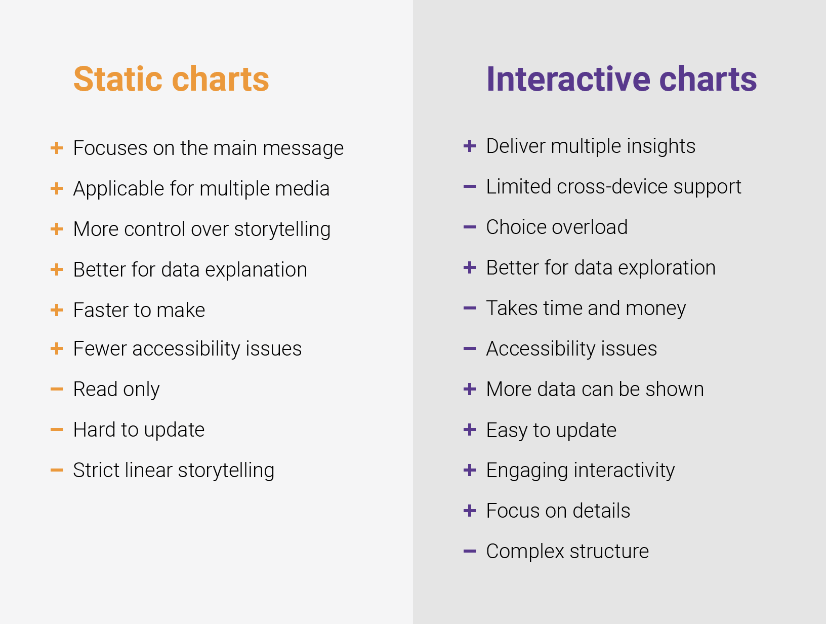
While static charts are useful, interactive visualizations empower users to explore data more deeply, uncover patterns, and gain personalized insights. Altair is a Python library that excels at creating a wide range of interactive statistical visualizations with a concise and intuitive syntax.
2.1. Beyond Static: The Power of Interaction
- Why Interactive? Interactive visualizations allow users to explore data dynamically through features like tooltips, zooming, panning, and selections. This enhances engagement, facilitates the understanding of complex datasets, and enables users to ask their own questions of the data. <!---
- Interactivity transforms the audience from passive viewers into active data explorers.
- For example, hovering over a data point to see detailed information (tooltip), or selecting a subset of data to see it highlighted in other linked charts. --->
2.2. Introduction to Altair
- What is Altair? Altair is a declarative statistical visualization library for Python, built on top of Vega-Lite. "Declarative" means you specify what you want to visualize (the mapping from data to visual properties), rather than detailing how to draw it step-by-step (imperative). <!---
- Vega-Lite is a high-level visualization grammar, and Altair provides a Python API to generate Vega-Lite JSON specifications. These JSON specs are then rendered by JavaScript libraries in environments like Jupyter notebooks, web browsers, or MkDocs sites. --->
- Key Principles (Grammar of Graphics): Altair follows the Grammar of Graphics, a formal system for describing statistical graphics. Visualizations are built by mapping data columns to visual properties (encodings) of geometric shapes (marks). The core components are:
- Data: The dataset, typically a Pandas DataFrame. Altair works best with data in a "tidy" long-form format.
- Mark: The geometric object representing data (e.g.,
mark_point(),mark_bar(),mark_line(),mark_area(),mark_rect()). - Encoding: The mapping of data fields (columns) to visual channels like:
x: x-axis position (e.g., time, category)y: y-axis position (e.g., value, count)color: mark color (e.g., category, group)size: mark size (e.g., magnitude, importance)shape: mark shape (e.g., type, status)opacity: mark transparencytooltip: information to show on hover (e.g., ID, details) <!---
- The Grammar of Graphics provides a structured way to think about and construct visualizations, promoting consistency and expressiveness.
- Tidy data means each variable forms a column, each observation forms a row, and each type of observational unit forms a table. --->
- Benefits: This approach leads to:
- Concise Code: Complex charts can often be expressed in just a few lines of Python.
- Aesthetically Pleasing Defaults: Altair charts generally look good out-of-the-box.
- Powerful Interactivity: Built-in support for selections, tooltips, panning, and zooming.
- Comparison (Briefly):
plotnineis another Python library based on the Grammar of Graphics (an implementation of R'sggplot2). It shares the declarative philosophy with Altair.- Both Altair and
plotninecontrast with the more imperative (step-by-step drawing commands) approach of basicmatplotlib. Whilematplotlibis highly flexible and powerful, creating complex, publication-quality charts can require more verbose code. <!--- - The choice between Altair and plotnine can depend on familiarity with ggplot2 syntax (for plotnine users) or preference for Vega-Lite's interactivity and web-native output (for Altair users). --->
2.3. Basic Altair: Building Blocks
Let's look at the fundamental components for creating an Altair chart.
- Reference Card:
altair.Chart- Core Object:
alt.Chart(data): This is the starting point. You pass your Pandas DataFrame to it. <!---altis the conventional alias forimport altair as alt. --->
- Mark Type:
.mark_type(): Specifies the geometric shape. Examples:mark_point(): For scatter plots (e.g., correlations).mark_bar(): For bar charts (e.g., counts).mark_line(): For line charts (e.g., trends).mark_area(): For area charts (e.g., cumulative values).mark_rect(): For heatmaps (e.g., patterns).
- Encodings:
.encode(...): This is where you map data columns to visual properties.- Syntax:
channel='column_name:type_shorthand' - Type Shorthands:
:Q- Quantitative (continuous numerical data):N- Nominal (discrete, unordered categorical data):O- Ordinal (discrete, ordered categorical data):T- Temporal (date/time data)
- Example:
alt.X('age:Q'),alt.Y('value:Q'),alt.Color('category:N')<!--- - Specifying the correct data type is crucial for Altair to apply appropriate scales, axes, and legends. --->
- Syntax:
- Properties:
.properties(...): To set overall chart attributes.width=W(integer, pixels)height=H(integer, pixels)title='My Chart Title'
- Interactivity:
.interactive(): A convenient shortcut to enable basic panning and zooming. - Saving Charts:
.save('filename.ext')'chart.html': Saves as a self-contained HTML file.'chart.json': Saves the Vega-Lite JSON specification. This is very useful for embedding in web pages or using with tools like MkDocs and Dash.'chart.png'or'chart.svg': Saves as a static image. Requires thevl-convertpackage (pip install vl-convert-python). <!---altair_vieweris another package that can help display charts during development, especially outside of Jupyter environments. --->
- Core Object:
-
Minimal Example (Scatter Plot): Let's assume we have a Pandas DataFrame
data_dfwith columns likex,y, andcategory.import altair as alt import pandas as pd # Example: Create a placeholder DataFrame if data_df is not loaded # This is just for demonstration if you run this code block standalone. # In a real scenario, data_df would be loaded from a CSV or other source. if 'data_df' not in locals(): data_df = pd.DataFrame({ 'x': [1, 2, 3, 4, 5, 6, 7, 8], 'y': [2, 4, 6, 8, 10, 12, 14, 16], 'id': ['A001', 'A002', 'A003', 'A004', 'A005', 'A006', 'A007', 'A008'], 'category': ['Type A', 'Type B', 'Type A', 'Type B', 'Type A', 'Type B', 'Type A', 'Type B'] }) scatter_plot = alt.Chart(data_df).mark_point(size=100).encode( x='x:Q', # X-axis, quantitative y='y:Q', # Y-axis, quantitative color='category:N', # Color points by category (nominal) tooltip=['id:N', 'x:Q', 'y:Q', 'category:N'] # Info on hover ).properties( title='X vs. Y by Category' ).interactive() # Enable pan and zoom # To display in a Jupyter Notebook, this is often enough: # scatter_plot # To save (uncomment the one you need): # scatter_plot.save('x_vs_y_scatter.html') # scatter_plot.save('x_vs_y_scatter.json') # scatter_plot.save('x_vs_y_scatter.png') # Requires vl-convert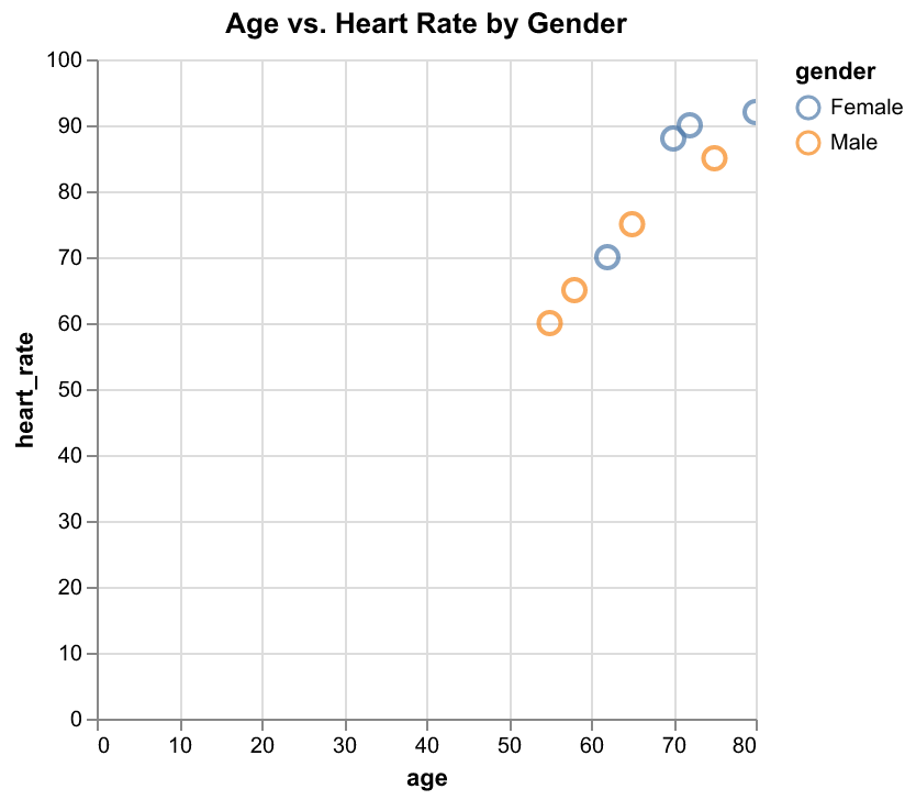
-
Generated JSON Specification: When you save this chart as JSON (
scatter_plot.save('chart.json')), Altair generates a Vega-Lite specification like this:<!---{ "$schema": "https://vega.github.io/schema/vega-lite/v5.20.1.json", "data": { "name": "data-cc85da6ba14ea85607962b8b20b8f7ab" }, "mark": { "type": "point", "size": 100 }, "encoding": { "x": {"field": "x", "type": "quantitative"}, "y": {"field": "y", "type": "quantitative"}, "color": {"field": "category", "type": "nominal"}, "tooltip": [ {"field": "id", "type": "nominal"}, {"field": "x", "type": "quantitative"}, {"field": "y", "type": "quantitative"}, {"field": "category", "type": "nominal"} ] }, "title": "X vs. Y by Category", "params": [ { "name": "param_1", "select": {"type": "interval", "encodings": ["x", "y"]}, "bind": "scales" } ], "datasets": { "data-cc85da6ba14ea85607962b8b20b8f7ab": [ {"x": 1, "y": 2, "id": "A001", "category": "Type A"}, {"x": 2, "y": 4, "id": "A002", "category": "Type B"} ] } }- This JSON specification is what gets embedded in MkDocs sites and Dash apps.
- Understanding this structure helps debug issues and customize charts beyond Python.
- The "params" section handles the interactivity from
.interactive(). - Notice how Altair separates the data into a "datasets" section and references it by name. --->
2.4. Building Blocks for Dynamic Charts (e.g., for Interactive Dashboard)
To create more advanced interactive charts, like the dashboard we'll aim for in the Dash demo, we need a few more Altair concepts. This section focuses on the Altair techniques for creating components that can be assembled into such visualizations.
- Selections: Selections are the core of Altair's interactivity. They define how users can interact with the chart.
alt.selection_interval(): Allows selecting a rectangular region (brushing).alt.selection_point(): Allows selecting single or multiple discrete points.alt.selection_single(): Allows selecting a single discrete item, often used withbindfor widgets.
- Input Binding (for
selection_single): Connects a selection to an HTML input element.bind=alt.binding_range(min=V, max=V, step=V): Creates a slider.bind=alt.binding_select(options=[...]): Creates a dropdown menu.
- Conditional Encodings: Change visual properties based on a selection.
alt.condition(selection, value_if_selected, value_if_not_selected)- Example:
color=alt.condition(my_selection, 'steelblue', 'lightgray')
- Transformations: Modify the data before encoding.
transform_filter(selection_or_expression): Filter data based on a selection or a Vega expression.transform_aggregate(...): Perform aggregations (e.g., mean, sum).transform_window(...): For window functions (e.g., rank, cumulative sum).
-
Layering & Concatenation: Combine multiple chart specifications.
chart1 + chart2: Layer charts on top of each other (share axes).chart1 | chart2: Place charts side-by-side (horizontal concatenation).chart1 & chart2: Place charts one above the other (vertical concatenation).
-
Key Altair features for an interactive dashboard:
- Data: A DataFrame with columns for metrics, categories, and timestamps.
- Time Slider: Use
alt.selection_singlewithbind=alt.binding_rangeto create a slider for thetimestampfield. - Filtering: Use
transform_filter(timestamp_slider_selection)to filter the data displayed in the chart based on the time selected by the slider. - Encodings: Map the data columns to
x,y,size, andcolorvisual channels. - Tooltips: Provide rich information on hover.
- Scales: May need to customize scales (e.g.,
alt.Scale(type="log")for skewed distributions).
-
Example Pattern for Dynamic Charts:
# Basic pattern for time-based filtering
time_slider = alt.selection_single(
    fields=['timestamp'],
    bind=alt.binding_range(min='2024-01-01', max='2024-12-31', step=86400000)  # 1 day in milliseconds
)

chart = alt.Chart(data).mark_circle().encode(
    x='timestamp:T',
    y='value:Q',
    size='magnitude:Q',
    color='category:N'
).add_params(time_slider).transform_filter(time_slider)
Pro Tip for Data Scientists: 📊 When creating interactive visualizations with Altair, consider these encoding strategies: * X-axis: Time or category * Y-axis: Value or count * Size: Magnitude or importance * Color: Category or status * Animation: Time progression showing trends
Demo 2: Interactive Altair Chart
- (Refer to
lectures/09/demo/02_altair_interactive_chart.md) <!---- This demo will involve creating a simpler interactive chart, perhaps with a categorical filter or a brush selection, using a real dataset.
- It reinforces the concepts of selections and saving for embedding. --->
2.5. Controlling Interactivity
Altair provides fine-grained control over interactive features. Here are some key controls:
-
Disabling Specific Interactions:
-
Selection Types:
alt.selection_interval(): For rectangular region selectionalt.selection_point(): For selecting individual pointsalt.selection_single(): For single item selection
2.6. Health Data Visualization Examples
Here are several examples of health data visualizations using Altair, each with its reference card and code:
1. Basic Scatter Plot
Reference Card: alt.Chart().mark_circle() - Purpose: Visualize relationships between two continuous variables - Key Parameters: - x: Quantitative variable (e.g., age) - y: Quantitative variable (e.g., blood pressure) - color: Categorical variable for grouping - tooltip: Fields to show on hover
Code:
scatter = alt.Chart(df).mark_circle().encode(
    x='age:Q',
    y='blood_pressure:Q',
    color='condition:N',
    tooltip=['patient_id:N', 'age:Q', 'blood_pressure:Q', 'condition:N']
).properties(
    title='Age vs Blood Pressure by Condition',
    width=400,
    height=300
)
Chart:
2. Time Series Plot
Reference Card: alt.Chart().mark_line() - Purpose: Show trends over time - Key Parameters: - x: Temporal variable (e.g., visit date) - y: Quantitative variable (e.g., blood pressure) - color: Categorical variable for grouping - tooltip: Fields to show on hover
Code:
time_series = alt.Chart(df).mark_line().encode(
    x='visit_date:T',
    y='blood_pressure:Q',
    color='condition:N',
    tooltip=['visit_date:T', 'blood_pressure:Q', 'condition:N']
).properties(
    title='Blood Pressure Trends Over Time',
    width=600,
    height=300
)
Chart:
3. Box Plot
Reference Card: alt.Chart().mark_boxplot() - Purpose: Show distribution of continuous variables by category - Key Parameters: - x: Categorical variable (e.g., condition) - y: Quantitative variable (e.g., heart rate) - color: Categorical variable for grouping - tooltip: Fields to show on hover
Code:
box_plot = alt.Chart(df).mark_boxplot().encode(
    x='condition:N',
    y='heart_rate:Q',
    color='condition:N',
    tooltip=['condition:N', 'heart_rate:Q']
).properties(
    title='Heart Rate Distribution by Condition',
    width=400,
    height=300
)
Chart:
4. Heatmap
Reference Card: alt.Chart().mark_rect() - Purpose: Show relationships between two categorical variables - Key Parameters: - x: Categorical variable (e.g., condition) - y: Categorical variable (e.g., medication) - color: Aggregated quantitative variable (e.g., mean dosage) - tooltip: Fields to show on hover
Code:
heatmap = alt.Chart(df).mark_rect().encode(
    x=alt.X('condition:N', title='Condition'),
    y=alt.Y('medication:N', title='Medication'),
    color=alt.Color('mean(dosage):Q', title='Average Dosage'),
    tooltip=['condition:N', 'medication:N', 'mean(dosage):Q']
).properties(
    title='Average Medication Dosage by Condition',
    width=400,
    height=300
)
Chart:
5. Interactive Selection
Reference Card: alt.selection_point() - Purpose: Enable interactive filtering through legend - Key Parameters: - fields: Fields to filter on - bind: Where to bind the selection (e.g., 'legend') - condition: How to highlight selected data
Code:
selection = alt.selection_point(
    name='select',
    fields=['condition'],
    bind='legend'
)

interactive = alt.Chart(df).mark_circle().encode(
    x='age:Q',
    y='blood_pressure:Q',
    color=alt.condition(
        selection,
        'condition:N',
        alt.value('lightgray')
    ),
    tooltip=['patient_id:N', 'age:Q', 'blood_pressure:Q', 'condition:N']
).add_params(selection).properties(
    title='Interactive Patient Data',
    width=400,
    height=300
)
Chart:
6. Faceted Plot
Reference Card: alt.Chart().facet() - Purpose: Create small multiples for comparison - Key Parameters: - column: Variable to facet by - mark: Type of mark to use - encode: Visual encodings for each facet
Code:
faceted = alt.Chart(df).mark_bar().encode(
    x='medication:N',
    y='count():Q',
    color='condition:N',
    tooltip=['medication:N', 'count():Q', 'condition:N']
).facet(
    column='condition:N'
).properties(
    title='Medication Distribution by Condition',
    width=100,
    height=300
)
Chart:
2.7. Advanced Altair Examples
Scatter Plot with Marginal Histograms
Code:
import altair as alt
import pandas as pd
import numpy as np

# Generate sample data
np.random.seed(42)
df = pd.DataFrame({
    'x': np.random.normal(0, 1, 100),
    'y': np.random.normal(0, 1, 100),
    'category': np.random.choice(['A', 'B', 'C'], 100)
})

# Create the main scatter plot
scatter = alt.Chart(df).mark_circle().encode(
    x='x:Q',
    y='y:Q',
    color='category:N',
    tooltip=['x:Q', 'y:Q', 'category:N']
).properties(
    width=400,
    height=400
)

# Create the marginal histograms
x_hist = alt.Chart(df).mark_bar().encode(
    x=alt.X('x:Q', bin=True),
    y='count()'
).properties(
    width=400,
    height=100
)

y_hist = alt.Chart(df).mark_bar().encode(
    y=alt.Y('y:Q', bin=True),
    x='count()'
).properties(
    width=100,
    height=400
)

# Combine the charts
chart = (x_hist & (scatter | y_hist))
Chart:
Interactive Variable Selection
Code:
# Create a parameter for variable selection
var_select = alt.param(
    name='var_select',
    bind=alt.binding_select(
        options=['x', 'y', 'category'],
        name='Select Variable: '
    ),
    value='x'
)

# Create the chart with variable selection
chart = alt.Chart(df).mark_circle().encode(
    x=alt.X('x:Q'),
    y=alt.Y('y:Q'),
    color=alt.condition(
        var_select == 'category',
        'category:N',
        alt.value('steelblue')
    )
).add_params(var_select)
Chart:
Layered Chart with Multiple Marks
Code:
# Create a layered chart with points and a trend line
base = alt.Chart(df).encode(
    x='x:Q',
    y='y:Q'
)

points = base.mark_circle().encode(
    color='category:N',
    tooltip=['x:Q', 'y:Q', 'category:N']
)

trend = base.mark_line(color='red').transform_regression('x', 'y')

chart = (points + trend).properties(
    width=400,
    height=300,
    title='Scatter Plot with Trend Line'
)
Chart:
Interactive Brushing and Linking
Code:
# Create a selection for brushing
brush = alt.selection_interval()

# Create two linked scatter plots
chart1 = alt.Chart(df).mark_circle().encode(
    x='x:Q',
    y='y:Q',
    color=alt.condition(brush, 'category:N', alt.value('lightgray')),
    tooltip=['x:Q', 'y:Q', 'category:N']
).add_params(brush)

chart2 = alt.Chart(df).mark_circle().encode(
    x='category:N',
    y='y:Q',
    color=alt.condition(brush, 'category:N', alt.value('lightgray')),
    tooltip=['x:Q', 'y:Q', 'category:N']
).add_params(brush)

# Combine the charts
chart = (chart1 | chart2).properties(
    width=300,
    height=300
)
Chart:
Generated JSON Specification
When saved as JSON, these charts produce specifications like:
{
  "$schema": "https://vega.github.io/schema/vega-lite/v5.json",
  "data": {
    "name": "data"
  },
  "mark": "circle",
  "encoding": {
    "x": {"field": "x", "type": "quantitative"},
    "y": {"field": "y", "type": "quantitative"},
    "color": {"field": "category", "type": "nominal"}
  },
  "params": [
    {
      "name": "var_select",
      "bind": {
        "input": "select",
        "options": ["x", "y", "category"],
        "name": "Select Variable: "
      },
      "value": "x"
    }
  ]
}
Demo 3: Automated Report with MkDocs
- Location: The full project for this demo is located in
lectures/09/demo/mkdocs_report_project/. - Instructions: A detailed guide for setting up and running this demo, including explanations of the directory structure,
mkdocs.ymlconfiguration, chart generation script, GitHub Actions workflow, and report content, can be found inlectures/09/demo/03_mkdocs_project_guide.md. (This guide file will be created next, based on the old03_mkdocs_automated_report.md). - Key Features: This demo showcases a complete, self-contained MkDocs project that:
- Generates Altair charts via a Python script and saves them as JSON.
- Embeds these charts and Mermaid diagrams into Markdown pages using
mkdocs-charts-plugin. - Uses a professional theme (Material for MkDocs) with various features.
- Includes a GitHub Actions workflow for automated deployment to GitHub Pages. <!---
- This demo provides a comprehensive example of building and deploying an automated data science report. Students will explore the project structure and run the build process. --->
3.8. GitHub Setup for MkDocs
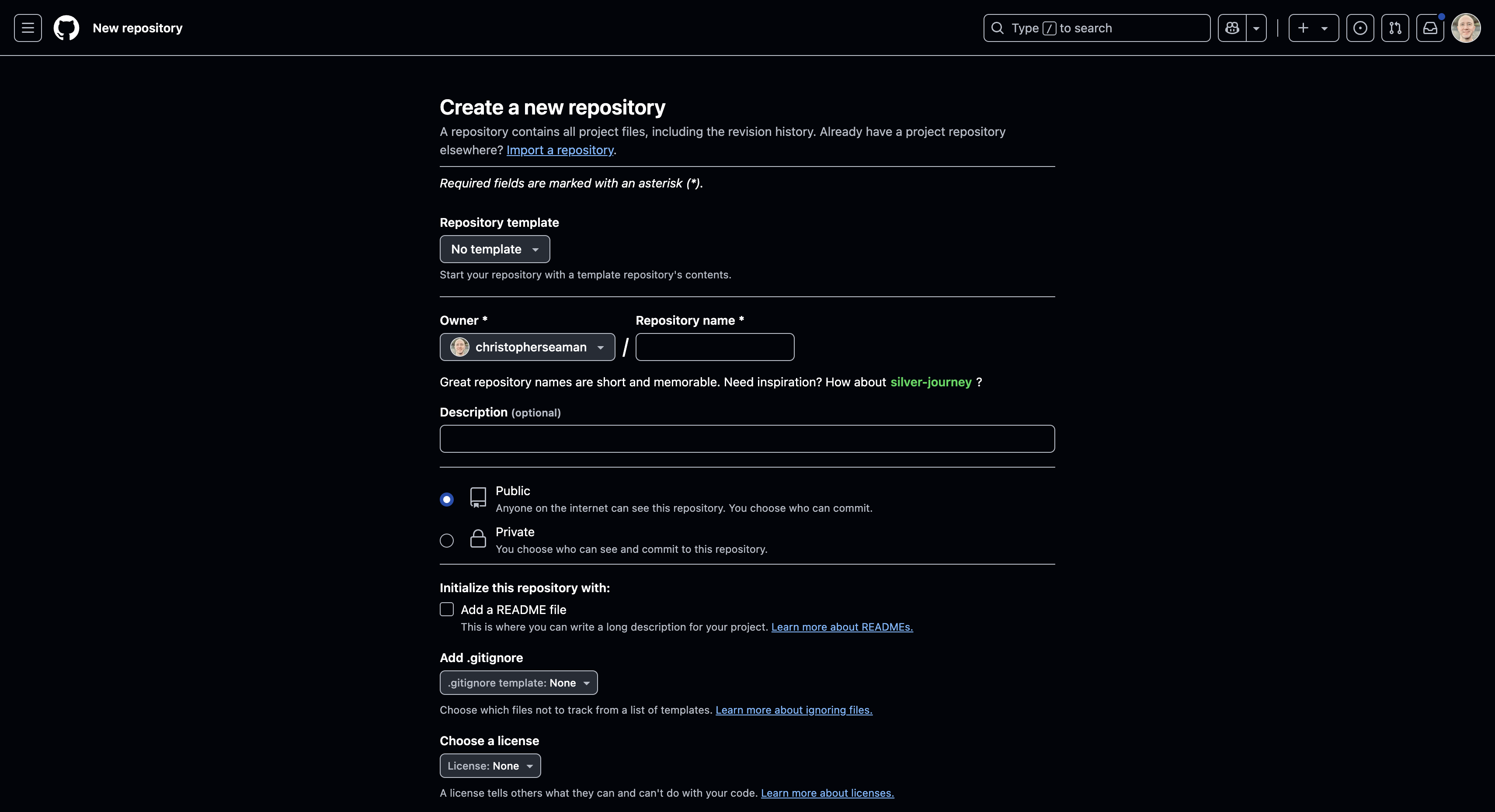
Step 1: Create a New Repository
- Go to GitHub.com and click the "+" button in the top right
- Select "New repository"
- Name your repository (e.g.,
health-docs) - Make it public
- Initialize with a README
Step 2: Clone and Setup
# Clone the repository
git clone https://github.com/yourusername/health-docs.git
cd health-docs

# Initialize MkDocs
mkdocs new .

# Install dependencies
pip install -r requirements.txt
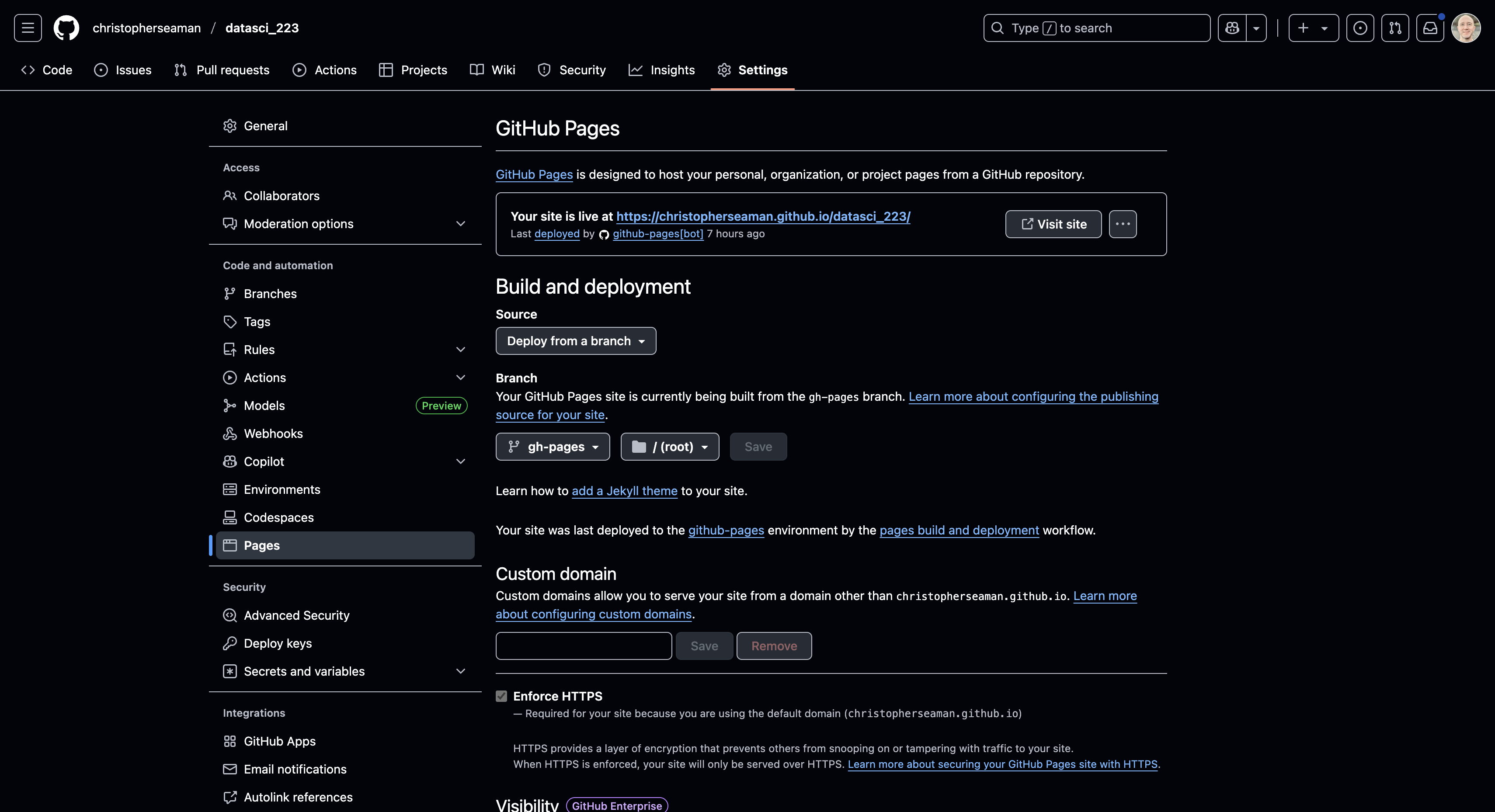
Step 3: Configure GitHub Pages
- Go to your repository's Settings
- Navigate to "Pages" in the sidebar
- Under "Source", select "GitHub Actions"
Step 4: Add GitHub Actions Workflow
Create .github/workflows/deploy.yml:
name: Deploy Docs
on:
  push:
    branches:
      - main
  pull_request:
    branches:
      - main

jobs:
  deploy:
    runs-on: ubuntu-latest
    steps:
      - uses: actions/checkout@v3
      - uses: actions/setup-python@v4
        with:
          python-version: 3.x
      - run: pip install mkdocs-material
      - run: mkdocs gh-deploy --force
Step 5: Verify Deployment
- Push your changes to GitHub
- Check the Actions tab to monitor deployment
- Once complete, your site will be available at
https://yourusername.github.io/health-docs/

Example: Published Documentation Site
Here's an example of a well-structured MkDocs site:
3.6. Useful MkDocs Plugins
Here are some essential plugins for data science reports:
-
mkdocs-charts-plugin- Embeds Vega-Lite charts in markdown
- Supports dark mode and instant loading
- Configuration:
plugins:
  - charts
extra_javascript:
  - https://cdn.jsdelivr.net/npm/vega@5
  - https://cdn.jsdelivr.net/npm/vega-lite@5
  - https://cdn.jsdelivr.net/npm/vega-embed@6
markdown_extensions:
  - pymdownx.superfences:
      custom_fences:
        - name: vegalite
          class: vegalite
          format: !!python/name:mkdocs_charts_plugin.fences.fence_vegalite
-
mkdocs-material- Rich feature set including:
- Search
- Tabs
- Code blocks with syntax highlighting
- Admonitions
- Task lists
- Configuration:
- Rich feature set including:
-
mkdocs-exporter- Generates PDF documents
- Supports custom page selection
- Configuration:
3.7. Deployment Options
GitHub Pages Deployment
-
Simple Branch Deployment
# .github/workflows/deploy.yml name: Deploy to GitHub Pages on: push: branches: [ main ] jobs: deploy: runs-on: ubuntu-latest steps: - uses: actions/checkout@v2 - uses: actions/setup-python@v2 with: python-version: 3.x - run: pip install mkdocs-material mkdocs-charts-plugin - run: mkdocs gh-deploy --force -
Custom Branch Deployment
# .github/workflows/deploy.yml
name: Deploy to GitHub Pages
on:
  push:
    branches: [ main ]
jobs:
  deploy:
    runs-on: ubuntu-latest
    steps:
      - uses: actions/checkout@v2
      - uses: actions/setup-python@v2
        with:
          python-version: 3.x
      - run: pip install -r requirements.txt
      - run: mkdocs build
      - name: Deploy
        uses: peaceiris/actions-gh-pages@v3
        with:
          github_token: ${{ secrets.GITHUB_TOKEN }}
          publish_dir: ./site
          publish_branch: gh-pages
Navigation Options
nav:
  - Home: index.md
  - Analysis:
    - Overview: analysis/overview.md
    - Methods: analysis/methods.md
    - Results: analysis/results.md
  - Visualizations:
    - Charts: visualizations/charts.md
    - Dashboards: visualizations/dashboards.md
  - About:
    - Team: about/team.md
    - Contact: about/contact.md
4. Interactive Dashboards with Dash by Plotly (20 minutes)
Dash by Plotly is a powerful framework for building analytical web applications. It's particularly well-suited for creating interactive dashboards that combine data visualization, user inputs, and real-time updates.
4.1. Why Dash for Dashboards?
- Concept & Benefits: Dash provides a framework for building web applications using Python. It's built on top of Flask and React, offering:
- Python-First: Write your entire application in Python, including the UI components.
- Interactive Components: Built-in support for interactive elements like dropdowns, sliders, and date pickers.
- Real-time Updates: Components can update in real-time based on user interactions or data changes.
- Responsive Design: Dash apps can be responsive and work well on different screen sizes.
- Production-Ready: Can be deployed to production servers and handle multiple users. <!---
- Dash is particularly powerful for data science applications because it allows you to create interactive UIs without needing to know JavaScript.
- The framework is mature and well-documented, making it a good choice for both beginners and experienced developers. --->
4.2. Basic Dash App Structure
-
Installation: First, install Dash and its dependencies:
* Minimal Example: Here's a basic Dash app that creates a simple scatter plot:import dash from dash import dcc, html import plotly.express as px import pandas as pd # Create sample data df = pd.DataFrame({ 'x': [1, 2, 3, 4, 5], 'y': [2, 4, 6, 8, 10], 'category': ['A', 'B', 'A', 'B', 'A'] }) # Initialize the Dash app app = dash.Dash(__name__) # Create the scatter plot fig = px.scatter(df, x='x', y='y', color='category', title='Sample Scatter Plot') # Define the app layout app.layout = html.Div([ html.H1('My First Dash App'), dcc.Graph(figure=fig) ]) # Run the app if __name__ == '__main__': app.run(debug=True)
4.3. Interactive Components
-
Input Components: Dash provides various input components that can trigger callbacks:
import dash
from dash import dcc, html
from dash.dependencies import Input, Output
import plotly.express as px
import pandas as pd

# Create sample data
df = pd.DataFrame({
    'x': [1, 2, 3, 4, 5],
    'y': [2, 4, 6, 8, 10],
    'category': ['A', 'B', 'A', 'B', 'A']
})

# Initialize the Dash app
app = dash.Dash(__name__)

# Define the app layout
app.layout = html.Div([
    html.H1('Interactive Dash App'),

    # Dropdown for selecting category
    html.Label('Select Category:'),
    dcc.Dropdown(
        id='category-dropdown',
        options=[{'label': cat, 'value': cat} for cat in df['category'].unique()],
        value='A'
    ),

    # Graph component
    dcc.Graph(id='scatter-plot')
])

# Define callback to update graph
@app.callback(
    Output('scatter-plot', 'figure'),
    [Input('category-dropdown', 'value')]
)
def update_graph(selected_category):
    filtered_df = df[df['category'] == selected_category]
    fig = px.scatter(filtered_df, x='x', y='y',
                    title=f'Scatter Plot for Category {selected_category}')
    return fig

# Run the app
if __name__ == '__main__':
    app.run(debug=True)
4.4. Advanced Features
-
Multiple Inputs/Outputs: Callbacks can have multiple inputs and outputs:
* State Management: Use@app.callback( [Output('graph1', 'figure'), Output('graph2', 'figure')], [Input('dropdown1', 'value'), Input('dropdown2', 'value')] ) def update_graphs(value1, value2): # Update logic for both graphs return fig1, fig2Statefor values that shouldn't trigger updates:* Interval Updates: Usefrom dash.dependencies import Input, Output, State @app.callback( Output('output', 'children'), [Input('button', 'n_clicks')], [State('input', 'value')] ) def update_output(n_clicks, input_value): # Only updates when button is clicked return f'Button clicked {n_clicks} times. Input value: {input_value}'dcc.Intervalfor periodic updates:
4.5. Deployment
-
Local Development: During development, use
* Production Deployment: For production, use a WSGI server like Gunicorn: * Cloud Deployment: Dash apps can be deployed to various cloud platforms: * Heroku: Create adebug=Truefor hot reloading:Procfilewithweb: gunicorn app:server* AWS Elastic Beanstalk: Use the Python platform * Google Cloud Run: Containerize the app and deploy to Cloud Run
Demo 4: Interactive Dashboard with Dash
- Location: The full project for this demo is located in
lectures/09/demo/dash_dashboard_project/. - Instructions: A detailed guide for setting up and running this demo, including explanations of the app structure, interactive components, callbacks, and deployment, can be found in
lectures/09/demo/04_dash_dashboard_guide.md. - Key Features: This demo showcases a complete Dash application that:
- Uses multiple interactive components (dropdowns, sliders, date pickers)
- Implements callbacks for real-time updates
- Includes responsive layout and styling
- Demonstrates deployment to a cloud platform <!---
- This demo provides a comprehensive example of building and deploying an interactive dashboard. Students will explore the app structure and run it locally. --->
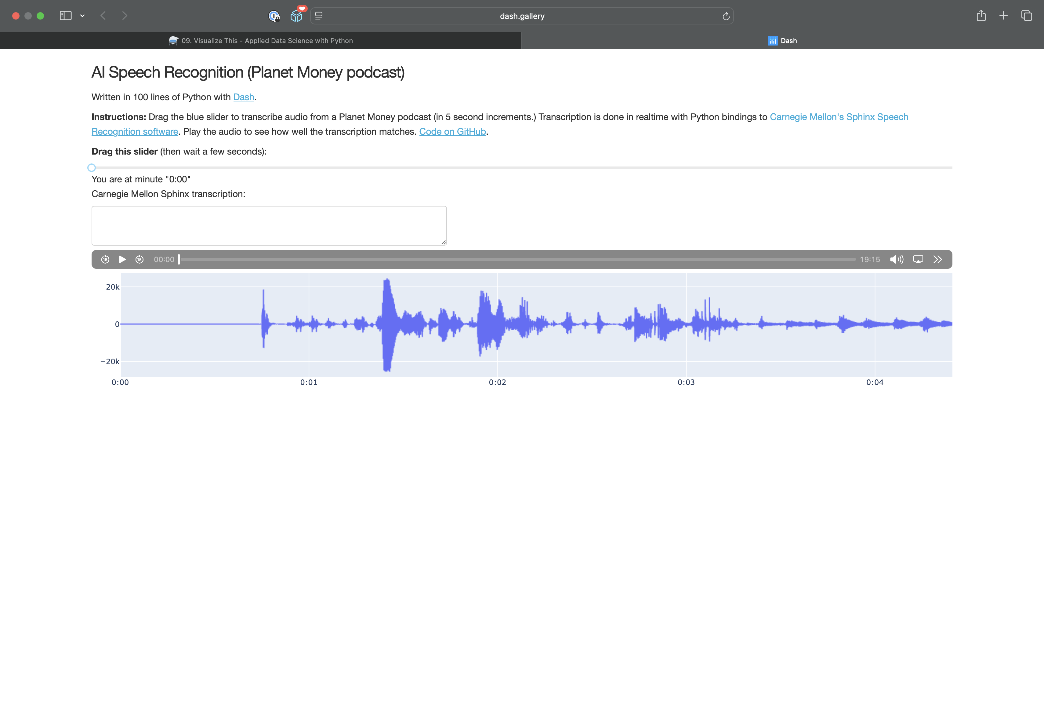
Dash Gallery Inspiration
Explore some of the most engaging and interactive Dash apps from the official Dash Gallery. These examples showcase what's possible with Dash for data science, health, and analytics communication:
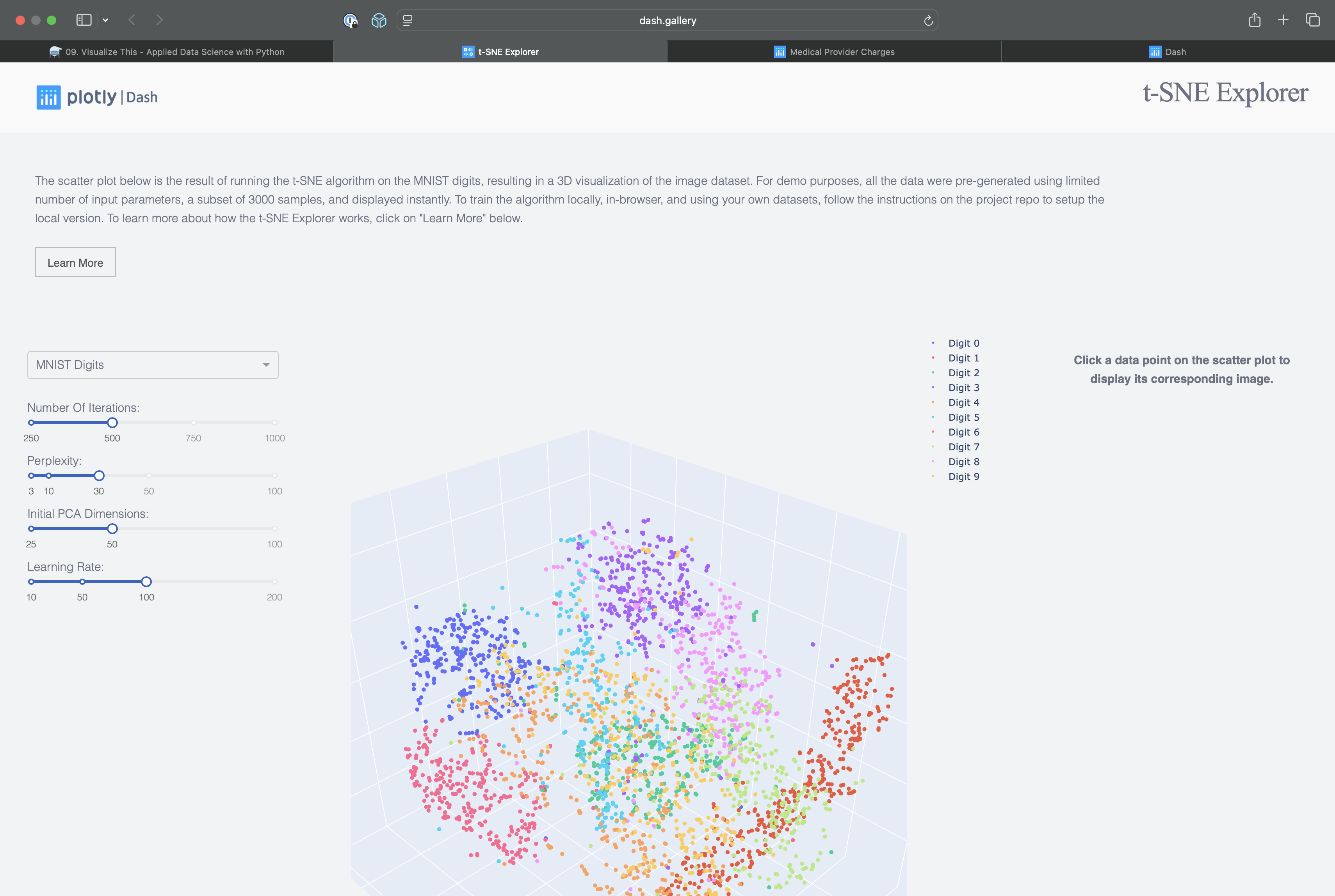
Visualizes high-dimensional data using t-SNE for interactive clustering and exploration.
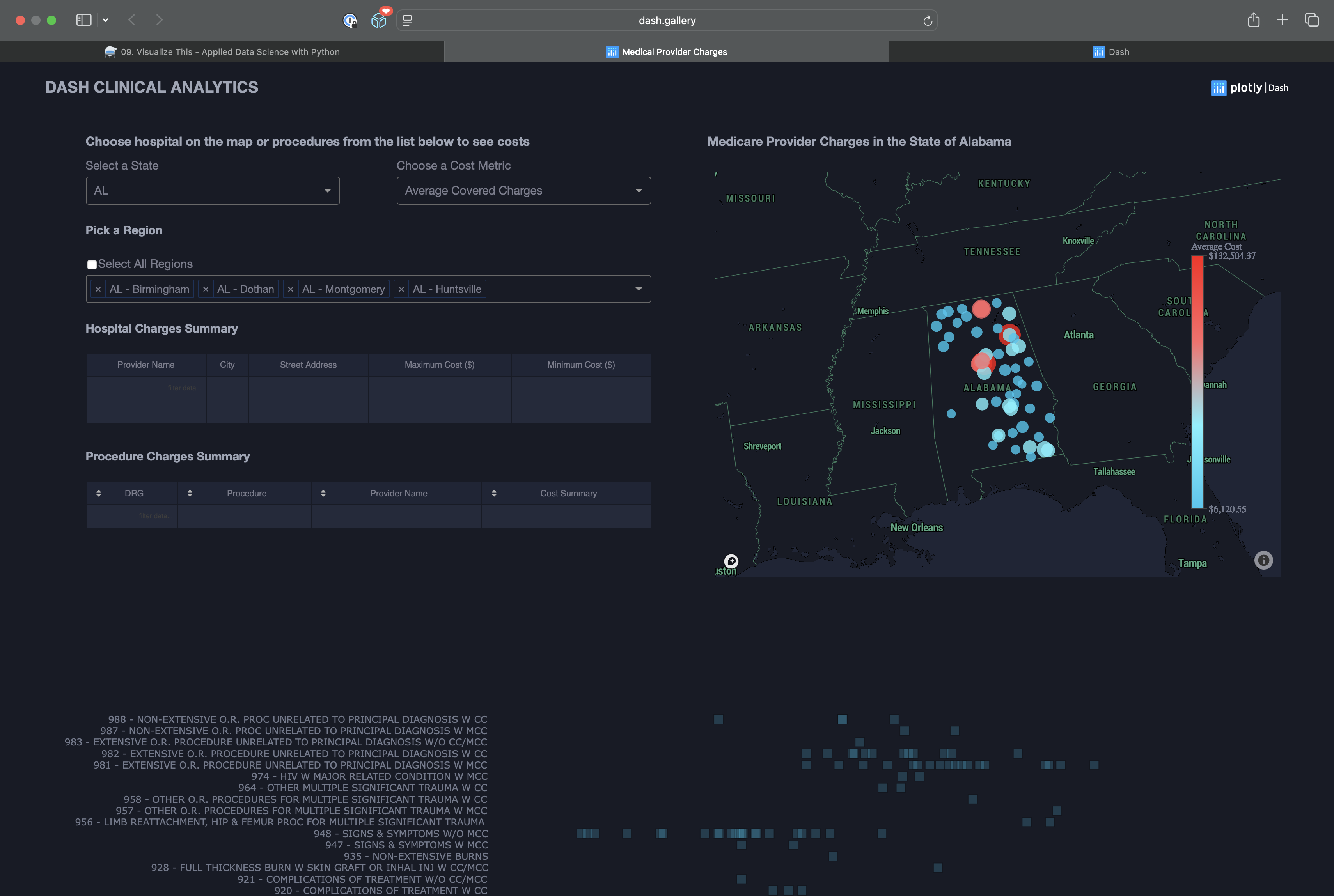
Interactive dashboard for exploring Medicare provider charges by state, region, and procedure.
Analyzes user behavior and engagement in web applications using Dash.
4.6. Data Handling in Dash
Base64 vs JSON
-
Base64 Encoding:
- Used for binary data (images, audio, files)
- Example:
-
JSON Data:
- Used for structured data (charts, tables)
- Example:
4.7. Simple Dashboard Example
Here's a simple dashboard with drill-down capabilities:
import dash
from dash import dcc, html
from dash.dependencies import Input, Output
import plotly.express as px
import pandas as pd

# Sample data
df = pd.DataFrame({
    'region': ['North', 'South', 'East', 'West'] * 3,
    'category': ['A', 'B', 'C'] * 4,
    'value': [10, 20, 30, 40, 50, 60, 70, 80, 90, 100, 110, 120]
})

# Initialize the app
app = dash.Dash(__name__)

# Layout
app.layout = html.Div([
    html.H1("Simple Dashboard"),

    # Region selector
    dcc.Dropdown(
        id='region-dropdown',
        options=[{'label': r, 'value': r} for r in df['region'].unique()],
        value='North'
    ),

    # Main chart
    dcc.Graph(id='main-chart'),

    # Drill-down chart
    dcc.Graph(id='drill-down-chart')
])

# Callbacks
@app.callback(
    [Output('main-chart', 'figure'),
     Output('drill-down-chart', 'figure')],
    [Input('region-dropdown', 'value')]
)
def update_charts(selected_region):
    # Filter data
    filtered_df = df[df['region'] == selected_region]

    # Main chart - bar plot by category
    main_fig = px.bar(
        filtered_df,
        x='category',
        y='value',
        title=f'Values by Category in {selected_region}'
    )

    # Drill-down chart - line plot over time
    drill_fig = px.line(
        filtered_df,
        x='category',
        y='value',
        title=f'Detailed View for {selected_region}'
    )

    return main_fig, drill_fig

if __name__ == '__main__':
    app.run(debug=True)